GW self-energy of a 2D square lattice Hubbard model
[1]:
import sys, os
import numpy as np
from triqs.plot.mpl_interface import plt,oplot

from h5 import HDFArchive
from triqs.atom_diag import *

from triqs.gf import *
from triqs.operators import c, c_dag, n, dagger
from itertools import product


from triqs.lattice.tight_binding import TBLattice
from triqs.lattice.utils import k_space_path

from triqs_tprf.lattice import lattice_dyson_g0_wk, lattice_dyson_g_wk, lattice_dyson_g0_fk, dynamical_screened_interaction_W, lattice_dyson_g_fk
from triqs_tprf.gw import bubble_PI_wk, gw_sigma, lindhard_chi00, g0w_sigma

from triqs_Nevanlinna import Solver

from triqs_maxent import *

import seaborn as sns
import scienceplots
plt.style.use(['science','notebook'])
sns.set_palette('muted')
Warning: could not identify MPI environment!
Starting serial run at: 2023-07-19 16:07:16.275962
Setup simple two orbital 2D Hubbard model on square lattice
[2]:
n_orb = 1

loc = np.zeros((n_orb,n_orb))
for i in range(n_orb):
    for j in range(n_orb):
        if i != 0 and i==j:
            loc[i,j] = -0.3
        if j > i or j < i:
            loc[i,j] = -0.5

t = -1.0 * np.eye(n_orb)   #nearest neighbor hopping
tp = 0.1 * np.eye(n_orb)    #next nearest neighbor hopping

hop= {  (0,0)  :  loc,
        (1,0)  :  t,
        (-1,0) :  t,
        (0,1)  :  t,
        (0,-1) :  t,
        (1,1)  :  tp,
        (-1,-1):  tp,
        (1,-1) :  tp,
        (-1,1) :  tp}

TB = TBLattice(units = [(1, 0, 0) , (0, 1, 0)], hoppings = hop, orbital_positions= [(0., 0., 0.)]*n_orb)
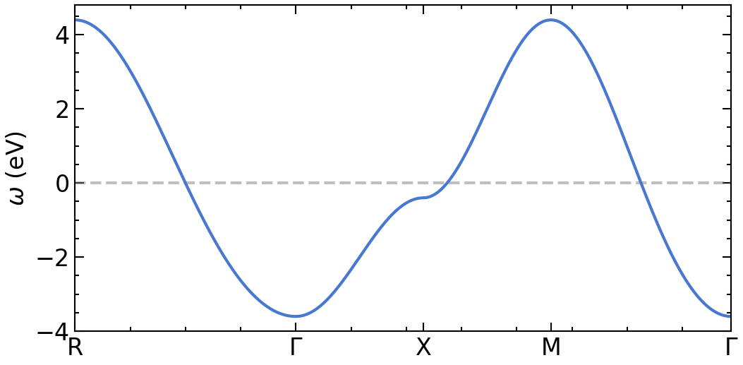
plot dispersion along high-symmetry lines
[3]:
n_pts = 101
G = np.array([ 0.00,  0.00,  0.00])
M = np.array([0.5, 0.5, 0.0])
X = np.array([0.5, 0.0, 0.0])
R = np.array([0.5, 0.5, 0.5])
paths = [(R, G), (G, X), (X, M), (M, G)]

kvecs, k  = k_space_path(paths, num=n_pts, bz=TB.bz)

e_mat = TB.fourier(kvecs)
e_val = TB.dispersion(kvecs)
eps_k = {'k': k, 'K': np.concatenate(([0],k[n_pts-1::n_pts])), 'eval': e_val, 'emat' : e_mat}
[4]:
fig, ax = plt.subplots(1,1, figsize=(8,4), dpi=150, squeeze=False)
ax = ax.reshape(-1)

for band in range(eps_k['eval'].shape[1]):
    ax[0].plot(eps_k['k'], eps_k['eval'][:,band].real, color='C0', zorder=2.5)

ax[0].axhline(y=0,zorder=2,color='gray',alpha=0.5,ls='--')
ax[0].set_xticks(eps_k['K'])
ax[0].set_xticklabels([r'R', '$\Gamma$', 'X', 'M', r'$\Gamma$'])
ax[0].set_xlim([eps_k['K'].min(), eps_k['K'].max()])
ax[0].set_ylabel(r'$\omega$ (eV)')

plt.show()
GW in imaginary time
[5]:
k_grid = (30,30,1)
k_mesh = TB.get_kmesh(n_k = k_grid)
e_k = TB.fourier(k_mesh)
eps_k = TB.dispersion(k_mesh)
mu = 0.

beta = 10
n_iw = 400
iw_mesh = MeshImFreq(beta=beta, S='Fermion', n_max=n_iw)
G0_iwk = lattice_dyson_g0_wk(mu=mu, e_k=e_k, mesh=iw_mesh)
setup bare interaction
[6]:
def construct_U_kan(n_orb, U, J, Up=None, Jc=None):

    orb_range = range(0, n_orb)
    U_kan = np.zeros((n_orb, n_orb, n_orb, n_orb))

    if not Up:
        Up = U-2*J
    if not Jc:
        Jc = J

    for i,j,k,l in product(orb_range, orb_range, orb_range, orb_range):
        if i == j == k == l: # Uiiii
            U_kan[i, j, k, l] = U
        elif i == k and j == l: # Uijij
            U_kan[i, j, k, l] = Up
        elif i == l and j == k: # Uijji
            U_kan[i, j, k, l] = J
        elif i == j and k ==l: # Uiijj
            U_kan[i, j, k, l] = Jc
    return U_kan
[7]:
U=1
Up=0.2
J=0.4
V_k = Gf(mesh=k_mesh, target_shape=[n_orb*1]*4)

V_bare = np.zeros((n_orb,n_orb,n_orb,n_orb))
# simple onsite intra orbital Coulomb repulsion
for i in range(n_orb):
    for j in range(n_orb):
        if i == j:
            V_bare[i,i,j,j] = U
        else:
            V_bare[i,i,j,j] = Up

V_bare = construct_U_kan(n_orb=n_orb,U=U,J=J,Up=Up)


V_k.data[:] = V_bare
Run one GW loop
[8]:
print('--> pi_bubble')
PI_iwk = bubble_PI_wk(G0_iwk)
print('--> screened_interaction_W')
Wr_iwk = dynamical_screened_interaction_W(PI_iwk, V_k)
print('--> gw_self_energy')
Σ_iwk = gw_sigma(Wr_iwk, G0_iwk)
print('--> lattice_dyson_g_wk')
G_wk = lattice_dyson_g_wk(mu, e_k, Σ_iwk)
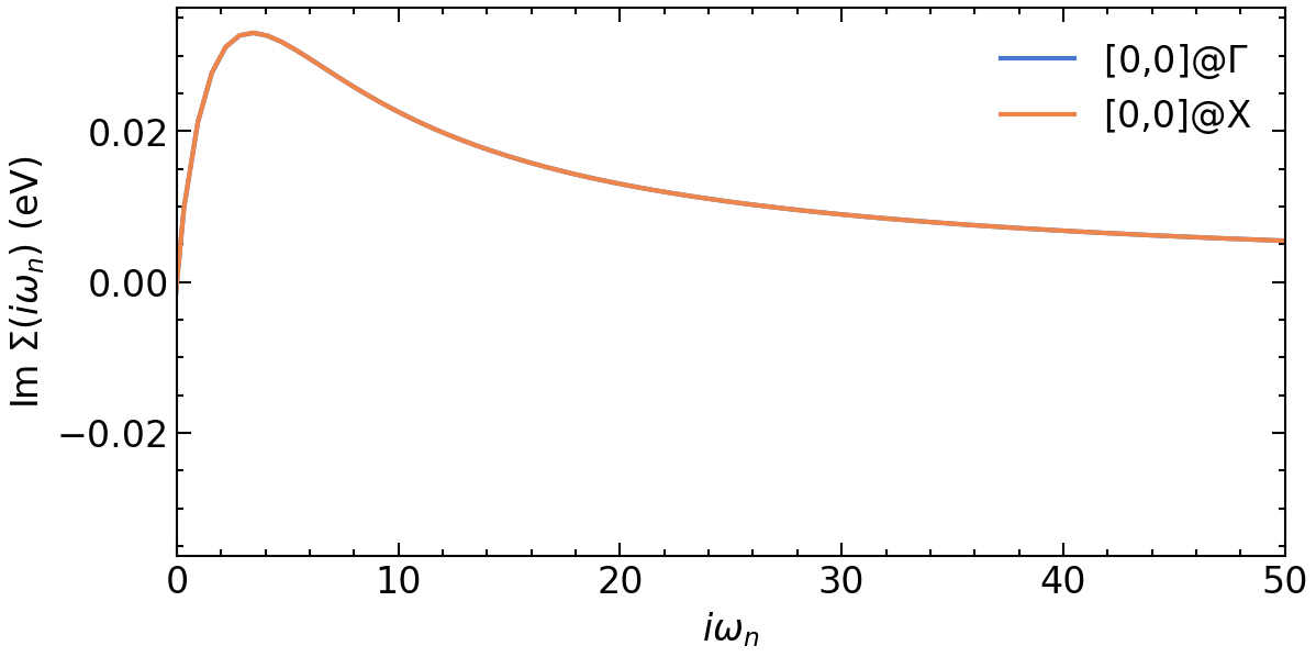
Σ_Γ_iw = Σ_iwk[:, Idx(0,0,0)]
Σ_X_iw = Σ_iwk[:, Idx(k_grid[1]-1,0,0)]
--> pi_bubble
--> screened_interaction_W
--> gw_self_energy
--> lattice_dyson_g_wk
Plot results
[25]:
fig, ax = plt.subplots(n_orb, n_orb, figsize=(8*n_orb,4*n_orb), dpi=150, squeeze=False,sharex=True)
ax = ax.reshape(-1)

ax[0].oplot(Σ_Γ_iw[i,j].imag, label=f'[{i},{j}]@$\Gamma$')
ax[0].oplot(Σ_X_iw[i,j].imag, label=f'[{i},{j}]@X')

ax[0].set_xlim(0,50)

ax[0].set_xlabel(r'$i\omega_n$')
ax[0].set_ylabel(r'Im $\Sigma (i\omega_n)$ (eV)')

plt.tight_layout(pad=0.4, w_pad=0.1, h_pad=0.4)
plt.show()
GW on real frequency axis
[10]:
# make sure 0 is not in the mesh! Divergence for q=[0,0,0]
# no large freq mesh is needed. kmesh critical for convergence here
n_w = 100
delta = 0.1
GW_window = (-15, 15)
w_mesh = MeshReFreq(window=GW_window, n_w=n_w)


G0_wk = lattice_dyson_g0_fk(mu=mu, e_k=e_k, mesh=w_mesh, delta=delta)
[11]:
print('--> pi_bubble')
PI_wk = lindhard_chi00(e_k=e_k, mesh=w_mesh, beta=beta, mu=mu, delta=delta)

print('--> screened_interaction_W')
Wr_wk = dynamical_screened_interaction_W(PI_wk, V_k)

print('--> gw_self_energy')
Σ_wk = g0w_sigma(mu=mu, beta=beta, e_k=e_k, W_fk=Wr_wk, v_k=V_k, delta=delta)

print('--> lattice_dyson_g_wk')
g_fk = lattice_dyson_g_fk(mu, e_k, Σ_wk, delta)

Σ_Γ_w = Σ_wk[:, Idx(0,0,0)]
Σ_X_w = Σ_wk[:, Idx(k_grid[1]-1,0,0)]
--> pi_bubble
--> screened_interaction_W
--> gw_self_energy
--> lattice_dyson_g_wk
Analytic continuation
Nevanlinna
[12]:
# setup Nevanlinna kernel solver
solver = Solver(kernel='CARATHEODORY')

# For the caratheodory formalism we have to subtract the Hartree shift
solver.solve(Σ_Γ_iw-Σ_Γ_iw(Σ_Γ_iw.mesh.last_index()))

Σ_w_mesh = MeshReFreq(window=GW_window, n_w=n_w*2)
Σ_Γ_w_CN = solver.evaluate(Σ_w_mesh, delta)
[13]:
# setup Nevanlinna kernel solver
solver = Solver(kernel='NEVANLINNA')

solver.solve(Σ_Γ_iw)

Σ_w_mesh = MeshReFreq(window=GW_window, n_w=n_w*2)
Σ_Γ_w_N = solver.evaluate(Σ_w_mesh, delta)
This is Nevanlinna analytical continuation. All off-diagonal elements will be ignored.
Pade
[14]:
Σ_Γ_w_P = Σ_Γ_w_N.copy()

Σ_Γ_w_P.set_from_pade(Σ_Γ_iw, n_points=n_iw, freq_offset=delta)
MaxEnt
[15]:
# Initialize SigmaContinuator
isc = DirectSigmaContinuator(Σ_Γ_iw)
[16]:
tm = TauMaxEnt()
tm.set_G_iw(isc.Gaux_iw)
tm.set_error(1.e-4)
tm.omega = HyperbolicOmegaMesh(omega_min=GW_window[0], omega_max=GW_window[1], n_points=300)
tm.alpha_mesh = LogAlphaMesh(alpha_min=1e-2, alpha_max=5e2, n_points=60)
result = tm.run()
print(('LineFit: ', result.analyzer_results['LineFitAnalyzer']['alpha_index']))
2023-07-19 16:08:15.167421
MaxEnt run
TRIQS application maxent
Copyright(C) 2018 Gernot J. Kraberger
Copyright(C) 2018 Simons Foundation
Authors: Gernot J. Kraberger and Manuel Zingl
This program comes with ABSOLUTELY NO WARRANTY.
This is free software, and you are welcome to redistributeit under certain conditions; see file LICENSE.
Please cite this code and the appropriate original papers (see documentation).

Minimal chi2: 2.780343854031604
scaling alpha by a factor 2401 (number of data points)
alpha[ 0] =   1.20050000e+06, chi2 =   1.86098288e+05, n_iter=      24
alpha[ 1] =   9.99352274e+05, chi2 =   1.47692183e+05, n_iter=       4
alpha[ 2] =   8.31907511e+05, chi2 =   1.17033657e+05, n_iter=       4
alpha[ 3] =   6.92518670e+05, chi2 =   9.25372230e+04, n_iter=       4
alpha[ 4] =   5.76484888e+05, chi2 =   7.29614636e+04, n_iter=       4
alpha[ 5] =   4.79892947e+05, chi2 =   5.73366261e+04, n_iter=       4
alpha[ 6] =   3.99485305e+05, chi2 =   4.48992104e+04, n_iter=       4
alpha[ 7] =   3.32550227e+05, chi2 =   3.50392785e+04, n_iter=       4
alpha[ 8] =   2.76830342e+05, chi2 =   2.72618500e+04, n_iter=       4
alpha[ 9] =   2.30446507e+05, chi2 =   2.11604692e+04, n_iter=       4
alpha[10] =   1.91834436e+05, chi2 =   1.63995950e+04, n_iter=       4
alpha[11] =   1.59691945e+05, chi2 =   1.27025481e+04, n_iter=       4
alpha[12] =   1.32935034e+05, chi2 =   9.84259729e+03, n_iter=       4
alpha[13] =   1.10661332e+05, chi2 =   7.63572391e+03, n_iter=       4
alpha[14] =   9.21196614e+04, chi2 =   5.93432811e+03, n_iter=       4
alpha[15] =   7.66847089e+04, chi2 =   4.62157117e+03, n_iter=       4
alpha[16] =   6.38359336e+04, chi2 =   3.60624447e+03, n_iter=       4
alpha[17] =   5.31400128e+04, chi2 =   2.81813049e+03, n_iter=       4
alpha[18] =   4.42362288e+04, chi2 =   2.20384925e+03, n_iter=       4
alpha[19] =   3.68243030e+04, chi2 =   1.72320364e+03, n_iter=       4
alpha[20] =   3.06542699e+04, chi2 =   1.34605178e+03, n_iter=       4
alpha[21] =   2.55180461e+04, chi2 =   1.04973179e+03, n_iter=       4
alpha[22] =   2.12424135e+04, chi2 =   8.17037947e+02, n_iter=       4
alpha[23] =   1.76831772e+04, chi2 =   6.34707643e+02, n_iter=       8
alpha[24] =   1.47203026e+04, chi2 =   4.92342240e+02, n_iter=       8
alpha[25] =   1.22538675e+04, chi2 =   3.81665508e+02, n_iter=       8
alpha[26] =   1.02006917e+04, chi2 =   2.96023756e+02, n_iter=       9
alpha[27] =   8.49153220e+03, chi2 =   2.30046214e+02, n_iter=       9
alpha[28] =   7.06874803e+03, chi2 =   1.79404997e+02, n_iter=       9
alpha[29] =   5.88435603e+03, chi2 =   1.40634238e+02, n_iter=       9
alpha[30] =   4.89841281e+03, chi2 =   1.10984285e+02, n_iter=       9
alpha[31] =   4.07766763e+03, chi2 =   8.82981124e+01, n_iter=      10
alpha[32] =   3.39444099e+03, chi2 =   7.09038537e+01, n_iter=      10
alpha[33] =   2.82569123e+03, chi2 =   5.75209700e+01, n_iter=      10
alpha[34] =   2.35223737e+03, chi2 =   4.71790688e+01, n_iter=      11
alpha[35] =   1.95811226e+03, chi2 =   3.91489212e+01, n_iter=      11
alpha[36] =   1.63002410e+03, chi2 =   3.28852039e+01, n_iter=      12
alpha[37] =   1.35690820e+03, chi2 =   2.79802902e+01, n_iter=      12
alpha[38] =   1.12955376e+03, chi2 =   2.41281131e+01, n_iter=      13
alpha[39] =   9.40293314e+02, chi2 =   2.10968320e+01, n_iter=      13
alpha[40] =   7.82744074e+02, chi2 =   1.87088142e+01, n_iter=      14
alpha[41] =   6.51592729e+02, chi2 =   1.68263626e+01, n_iter=      15
alpha[42] =   5.42416222e+02, chi2 =   1.53416958e+01, n_iter=      15
alpha[43] =   4.51532599e+02, chi2 =   1.41699055e+01, n_iter=      16
alpha[44] =   3.75876826e+02, chi2 =   1.32439023e+01, n_iter=      17
alpha[45] =   3.12897427e+02, chi2 =   1.25106661e+01, n_iter=      18
alpha[46] =   2.60470433e+02, chi2 =   1.19283627e+01, n_iter=      18
alpha[47] =   2.16827755e+02, chi2 =   1.14640737e+01, n_iter=      20
alpha[48] =   1.80497551e+02, chi2 =   1.10919855e+01, n_iter=      21
alpha[49] =   1.50254592e+02, chi2 =   1.07919377e+01, n_iter=      22
alpha[50] =   1.25078941e+02, chi2 =   1.05482575e+01, n_iter=      23
alpha[51] =   1.04121553e+02, chi2 =   1.03488142e+01, n_iter=      25
alpha[52] =   8.66756437e+01, chi2 =   1.01842507e+01, n_iter=      27
alpha[53] =   7.21528544e+01, chi2 =   1.00473564e+01, n_iter=      28
alpha[54] =   6.00634061e+01, chi2 =   9.93256293e+00, n_iter=      30
alpha[55] =   4.99995848e+01, chi2 =   9.83554893e+00, n_iter=      32
alpha[56] =   4.16219898e+01, chi2 =   9.75293868e+00, n_iter=      36
alpha[57] =   3.46480884e+01, chi2 =   9.68208054e+00, n_iter=      37
alpha[58] =   2.88426872e+01, chi2 =   9.62088520e+00, n_iter=      40
alpha[59] =   2.40100000e+01, chi2 =   9.56770438e+00, n_iter=      42
MaxEnt loop finished in 0:00:20.269188
('LineFit: ', 40)
[17]:
isc.set_Gaux_w_from_Aaux_w(result.analyzer_results['LineFitAnalyzer']['A_out'], result.omega, np_interp_A=n_w*2,
                           np_omega=n_w, w_min=GW_window[0], w_max=GW_window[1])

Σ_Γ_w_ME = isc.S_w
WARNING: the signature for all_reduce is now 'all_reduce(x, comm=world, op=MPI.SUM)'
        attempting compatibility with old signature
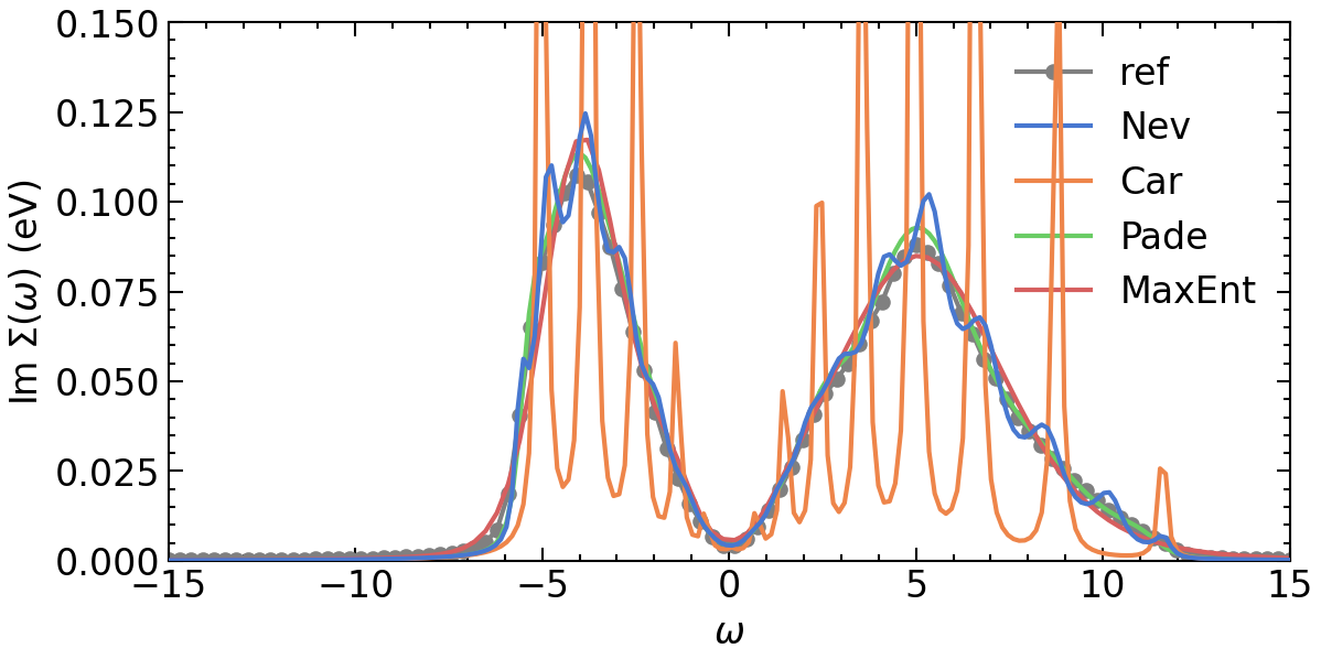
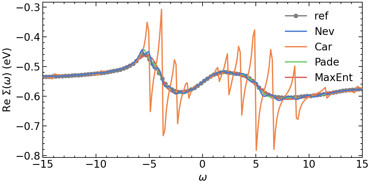
Comparison: Pade, Nevanlinna, Pade, and Maxent
[23]:
fig, ax = plt.subplots(n_orb, n_orb, figsize=(8*n_orb,4*n_orb), dpi=150, squeeze=False,sharex=True)
ax = ax.reshape(-1)

ax[0].oplot(Σ_Γ_w[i,j].imag, '-o', c='gray', label=f'ref')
ax[0].oplot(Σ_Γ_w_N[i,j].imag, label=f'Nev', zorder=10)
ax[0].oplot(Σ_Γ_w_CN[i,j].imag, label=f'Car', zorder=6)
ax[0].oplot(Σ_Γ_w_P[i,j].imag, label=f'Pade')
ax[0].oplot(Σ_Γ_w_ME[i,j].imag, label=f'MaxEnt')


ax[0].set_xlim(GW_window)
ax[0].set_ylim(0,0.15)

ax[0].set_xlabel(r'$\omega$')
ax[0].set_ylabel(r'Im $\Sigma (\omega)$ (eV)')


plt.tight_layout(pad=0.4, w_pad=0.1, h_pad=0.4)
plt.show()

fig, ax = plt.subplots(n_orb, n_orb, figsize=(8*n_orb,4*n_orb), dpi=150, squeeze=False,sharex=True)
ax = ax.reshape(-1)

# plotting results
ax[0].oplot(Σ_Γ_w[i,j].real, '-o', c='gray', label=f'ref')
ax[0].oplot(Σ_Γ_w_N[i,j].real, label=f'Nev', zorder=10)
ax[0].oplot((Σ_Γ_w_CN[i,j]+Σ_Γ_iw(Σ_Γ_iw.mesh.last_index())[i,j]).real, label=f'Car', zorder=6)
ax[0].oplot(Σ_Γ_w_P[i,j].real, label=f'Pade')
ax[0].oplot(Σ_Γ_w_ME[i,j].real, label=f'MaxEnt')

ax[0].set_xlim(GW_window)
ax[0].set_xlabel(r'$\omega$')
ax[0].set_ylabel(r'Re $\Sigma (\omega)$ (eV)')

plt.tight_layout(pad=0.4, w_pad=0.1, h_pad=0.4)
plt.show()