Charge self-consistent DFT+DMFT with VASP: SrVO₃

This tutorial walks through a full charge self-consistent (CSC) DFT+DMFT calculation for the prototypical correlated metal SrVO₃, using the VASP driver shipped with dftkit together with modest. We treat the vanadium \(t_{2g}\) manifold as the correlated subspace, solve the impurity problem with the CT-SEG solver from triqs_ctseg, and feed the resulting charge-density correction back into VASP until self-consistency.

SrVO₃ is the textbook moderately-correlated metal of DMFT: a single electron in the three vanadium \(t_{2g}\) orbitals (\(d^1\)) that, with a realistic \(U = 4.5\) eV and \(J = 0.65\) eV, develops a renormalized quasi-particle (\(Z \approx 0.6\)) on top of the DFT band structure. It stays metallic, which is exactly what the self-energy plot below shows.

Unlike the older vasp_dmft work flow, the whole calculation is driven by a single Python script: the dftkit VASP Driver keeps one VASP process alive in the background, exchanges the Kohn-Sham Hamiltonian, projectors and charge-density correction through the vaspout.h5 / vaspgamma.h5 interface, and runs the PLOVasp projector construction internally. No source-code patching and no auxiliary shell script are needed.

Note

This example requires VASP 6.5.0 or newer, built with HDF5 support enabled, plus the TRIQS applications triqs_modest, triqs_dftkit and triqs_ctseg.

All input files are collected in the tutorial directory: POSCAR, INCAR.scf, INCAR, plo.cfg, vasp_modest_csc.py and plot_sigma.py. You have to provide your own POTCAR (Sr_sv, V_sv and O).

Step 1 — converge the DFT charge density

We start from the simple cubic SrVO₃ cell:

SrVO3
 3.859374
 +1.00000000  +0.0000000000  +0.0000000000
 +0.0000000000  +1.00000000  +0.0000000000
 +0.0000000000  +0.0000000000  +1.0000000000
Sr V O
 1 1 3
Direct
 +0.0000000000  +0.0000000000  +0.0000000000
 +0.5000000000  +0.5000000000  +0.5000000000
 +0.5000000000  +0.5000000000  +0.0000000000
 +0.5000000000  +0.0000000000  +0.5000000000
 +0.0000000000  +0.5000000000  +0.5000000000

Run a plain DFT calculation first to obtain a converged charge density. We use the INCAR.scf below; the k-mesh is set automatically through KSPACING so no KPOINTS file is required.

System  = SrVO3

NCORE = 1
KPAR  = 4

ISMEAR = 0
SIGMA  = 0.1

KSPACING = 0.2

# converge the wave functions tightly
EDIFF  = 1.E-10
NELMIN = 20
NBANDS = 32

# energy window (absolute) in which the projector channels are optimized
EMIN  = -1.0
EMAX  = 10.1
NEDOS = 5001

LMAXMIX = 4

# project onto the vanadium d (t2g) states; atom 2 in the POSCAR is V
LORBIT  = 14
LOCPROJ = "2 : d : Pr"

LORBIT = 14 lets VASP optimize the localized projector channels inside the energy window defined by EMIN / EMAX, and the single LOCPROJ line selects the vanadium \(d\) states (atom 2 in the POSCAR). The projectors are written to vaspout.h5.

Run VASP in a dedicated directory and keep the resulting CHGCAR (and WAVECAR); the CSC run below reads them as its starting point.

Step 2 — the projector definition

The correlated subspace is configured for PLOVasp through plo.cfg:

[General]

[Group 1]
SHELLS = 1
NORMALIZE = True
EWINDOW = -1.4 2.0

[Shell 1]
LSHELL = 2
IONS = 2

TRANSFORM = 1.0  0.0  0.0  0.0  0.0
            0.0  1.0  0.0  0.0  0.0
            0.0  0.0  0.0  1.0  0.0

We define a single shell (LSHELL = 2, i.e. \(d\)) on the vanadium ion (IONS = 2) and normalize the projectors inside the energy window EWINDOW. The TRANSFORM matrix picks the three \(t_{2g}\) orbitals (\(d_{xy}, d_{yz}, d_{xz}\)) out of the five \(d\) orbitals, which are the only correlated degrees of freedom for cubic SrVO₃. The driver runs PLOVasp with this file on every charge iteration; you do not call the converter yourself.

Step 3 — switch the INCAR to charge self-consistency

For the CSC run we read the converged density and let VASP wait for the DMFT charge update at every electronic step:

System  = SrVO3

ISMEAR = 0
SIGMA  = 0.1

KSPACING = 0.2

# converge the wave functions
EDIFF = 1.E-7

# energy window (absolute) in which the projector channels are optimized
EMIN   = -1.0
EMAX   = 10.1
NBANDS = 32

LMAXMIX = 4

# project onto the vanadium d (t2g) states; atom 2 in the POSCAR is V
LORBIT  = 14
LOCPROJ = "2 : d : Pr"

# --- charge self-consistency -------------------------------------------------
# ICHARG = 5 makes VASP wait after every electronic step for the DMFT charge
# update and read it back, keeping the externally supplied density correction.
ICHARG = 5
NELM   = 1000
NELMIN = 1000
NELMDL = -3
IMIX   = 4
BMIX   = 0.2
AMIX   = 0.02

# exchange the projectors and the charge update through the HDF5 interface
# (vaspout.h5 / vaspgamma.h5); requires VASP >= 6.5.0 built with HDF5 support
LSYNCH5 = True

LWAVE = False
LCHG  = False

The key additions over the plain SCF run are ICHARG = 5 (read the charge density and apply the external correction), a very large NELM / NELMIN so that VASP never stops on its own, and the conservative mixing (IMIX/AMIX/BMIX) that stabilizes the charge update. LSYNCH5 = True routes the projectors and the charge-density correction through vaspout.h5 / vaspgamma.h5; from VASP 6.5.0 onwards this replaces the text-based GAMMA interface and needs no changes to the VASP source.

Copy the converged CHGCAR and WAVECAR from Step 1, this INCAR, the POSCAR, your POTCAR and plo.cfg into a fresh working directory.

Step 4 — the DMFT driver script

The complete CSC loop is implemented in vasp_modest_csc.py:

# ============================================================================
# Charge self-consistent (CSC) DFT+DMFT for SrVO3 with VASP + TRIQS/modest
# ============================================================================
#
# This script drives a full CSC DFT+DMFT calculation. The structure is two
# nested loops:
#
#   * outer loop (n_total_loops): one DFT charge update per iteration. VASP is
#     kept alive as a persistent background process by the dftkit VASP driver;
#     each outer iteration feeds the DMFT charge-density correction back into
#     VASP and reads the updated Kohn-Sham Hamiltonian / projectors.
#   * inner loop (n_dmft_loops): the DMFT self-consistency cycle (build the
#     hybridization, solve the impurity with CT-SEG, update the self-energy)
#     for the current DFT Hamiltonian.
#
# The run always ends on a DMFT step: after the last outer iteration the DFT
# code is not invoked again (see the guard around the charge update below).
#
# Required inputs in this directory: INCAR, POSCAR, POTCAR, KPOINTS and the
# PLOVasp projector definition plo.cfg.

import numpy as np

import triqs.utility.mpi as mpi

from triqs.gfs import BlockGf, MeshImFreq

from triqs_ctseg.solve_generic import solve_generic

import triqs_modest as M

from triqs_dftkit.vasp import Driver as VaspDriver, MPIHandler
from triqs_modest.dft_driver import DftDriver

from h5 import HDFArchive


# --- Physical and run parameters ---------------------------------------------
seedname = "vasp"
beta = 20.0          # inverse temperature (1/eV)
U    = 4.50          # Kanamori intra-orbital interaction (eV)
J    = 0.65          # Hund's coupling (eV)
Up   = U -2*J        # inter-orbital interaction (rotationally invariant choice)
n_iw = 1000          # number of Matsubara frequencies
n_total_loops = 10    # outer CSC (DFT charge) iterations
n_dmft_loops  =  1   # inner DMFT iterations per outer loop
n_iter_dft    =  2   # VASP SCF steps per outer loop (>1 for ALGO that needs
                     # several charge updates before DMFT; Sigma is held fixed
                     # and the charge correction is recomputed between steps)

# --- DFT driver --------------------------------------------------------------
# Wrap the dftkit VASP driver in the modest DftDriver. The VASP driver launches
# vasp_command under MPI and converts the output via PLOVasp (plo.cfg).
driver = DftDriver(VaspDriver(seedname=seedname, plo_cfg="plo.cfg",
                               mpi_handler=MPIHandler(mpi_exec="mpirun -np 16"),
                               vasp_command="vasp_std"))

# Run the initial DFT, convert the output, and return the target electron count
# together with the one-body elements (Kohn-Sham Hamiltonian + projectors).
target_density, obe = driver.one_body_elements_from_dft()
mpi.report(obe)

# Build the embedding (correlated subspace) from the projector space.
E = M.make_embedding(obe.C_space); mpi.report(E.description(True))

# Local Kanamori interaction Hamiltonian on the impurity.
h_int = M.make_kanamori(E.sigma_names, E.imp_decomposition(0), U, Up, J, False, False)

# Double-counting correction (Held's fully-localized-limit flavour).
DcTerm = M.DcSolver("NonPolarized", "cHeld", U, J)

mesh = MeshImFreq(beta=beta, S = "Fermion", n_iw=n_iw)

# DFT-only chemical potential and local Green's function, used to detect the
# degenerate block structure that the impurity quantities are symmetrized over.
mu_dft = M.find_chemical_potential(target_density, obe, beta, verbosity=False)
Gdft = E.extract(M.local_gf.gloc(mesh, obe, mu_dft))[0]
mpi.report(f"Gdft density= {Gdft.total_density().real}")

deg_blocks = M.analyze_degenerate_blocks(Gdft)
mpi.report(f"deg_blocks= {deg_blocks}")

# Initialise the self-energy: zero dynamic part plus the static double counting.
Sigma_imp_dc = DcTerm.dc_self_energy(Gdft)

Sigma_imp_dynamic, Sigma_imp_static = E.make_zero_imp_self_energies(mesh)[0]
for i in range(len(Sigma_imp_static)): Sigma_imp_static[i] += Sigma_imp_dc[i]

# DFT + DMFT loop
try:
    for n_iter in range(n_total_loops):
        mpi.report(f"\n{'='*60}\n=== Global DFT+DMFT iteration {n_iter+1}/{n_total_loops} ===\n{'='*60}")

        Hloc0 = E.extract(M.atomic_levels_and_delta.impurity_levels(obe))[0]
        mpi.report(f"Hloc0= {[h[0,0].real for h in Hloc0]}")

        # for first iteration converge Sigma imp first
        if n_iter == 0:
            n_dmft_loops_loc = 4
        else:
            n_dmft_loops_loc = n_dmft_loops
        # Begin DMFT loop
        for n_dmft_iter in range(n_dmft_loops_loc):
            mpi.report(f"\n--- DMFT iteration {n_dmft_iter+1}/{n_dmft_loops_loc} "
                       f"(global iter {n_iter+1}/{n_total_loops}) ---")

            Sigma_imp_static_minus_dc = [block-dc for (block, dc) in zip(Sigma_imp_static, Sigma_imp_dc)]

            Sigma_C_dynamic, Sigma_C_static = E.embed([Sigma_imp_dynamic], [Sigma_imp_static_minus_dc])

            mu = M.find_chemical_potential(target_density, obe, Sigma_C_dynamic, Sigma_C_static)

            Gloc = E.extract(M.local_gf.gloc(obe, mu, Sigma_C_dynamic, Sigma_C_static))[0]

            Eimp = [h-mu*np.eye(h.shape[0])-dc for (h,dc) in zip(Hloc0, Sigma_imp_dc)]

            Delta = M.symmetrize(M.hybridization(Eimp, Gloc, Sigma_imp_dynamic, Sigma_imp_static), deg_blocks)

            solver_params = dict(n_iw=n_iw, n_tau=10*n_iw, length_cycle=50,
                                 n_cycles = int(4e+6/mpi.size),
                                 n_warmup_cycles = int(1e+4),
                                 perform_tail_fit=True,
                                 fit_min_w=10, fit_max_w=14,
                                 )
            solver_results = solve_generic(Delta, Eimp, h_int, **solver_params)

            Sigma_imp_dynamic, Sigma_imp_static = solver_results.Sigma_dynamic, solver_results.Sigma_HartreeFock

            solver_results.G_iw         <<  M.symmetrize(solver_results.G_iw,          deg_blocks)
            solver_results.Sigma_iw     <<  M.symmetrize(solver_results.Sigma_iw,      deg_blocks)
            solver_results.Sigma_dynamic << M.symmetrize(solver_results.Sigma_dynamic, deg_blocks)
        # End of DMFT loop
        # Update Double-counting Term
        Sigma_imp_dc = DcTerm.dc_self_energy(solver_results.G_iw)
        Eimp_dc      = DcTerm.dc_energy(solver_results.G_iw)

        Sigma_imp_static_minus_dc = [block-dc for (block, dc) in zip(Sigma_imp_static, Sigma_imp_dc)]

        # Re-embed the self-energy
        Sigma_C_dynamic, Sigma_C_static = E.embed([Sigma_imp_dynamic], [Sigma_imp_static_minus_dc])

        # Re-compute the chemical potential
        mu = M.find_chemical_potential(target_density, obe, Sigma_C_dynamic, Sigma_C_static)

        # Compute the charge density correction
        N_k = M.charge_density_correction(obe, mu, Sigma_C_dynamic, Sigma_C_static)

        # Impurity interaction energy
        Eint = 0.5 * np.real((solver_results.Sigma_iw*solver_results.G_iw).total_density())
        mpi.report(f"Eint= {Eint}")
        Eint_m_dc = (Eint - Eimp_dc)
        mpi.report(f"Eint-Edc= {Eint_m_dc}")

        mpi.report("Saving DFT + DMFT iteration...")
        if mpi.is_master_node():
            with HDFArchive("checkpoint.h5", "a") as ar:
                path = f"it={len(ar) + 1}"
                ar.create_group(path)
                ar[path]["mu"]              = mu
                ar[path]["nloc"]            = Gloc.total_density().real
                ar[path]["nimp"]            = solver_results.G_iw.total_density().real
                ar[path]["Delta_iw"]        = Delta
                ar[path]["Eimp"]            = Eimp
                ar[path]["Gloc_iw"]         = Gloc
                ar[path]["Gimp_iw"]         = solver_results.G_iw
                ar[path]["Sigma_iw"]        = solver_results.Sigma_iw
                ar[path]["Sigma_iw_static"] = solver_results.Sigma_HartreeFock
                ar[path]["Sigma_dc"]        = Sigma_imp_dc

        # Update the one-body Hamiltonian with the charge density correction.
        # Skip on the last outer iteration: the calculation must end on a DMFT
        # step, so there is no point triggering another VASP charge update whose
        # result would never be used.
        if n_iter < n_total_loops - 1:
            mpi.report(f"Calling VASP charge update / DFT driver "
                       f"(global iter {n_iter+1}/{n_total_loops})...")
            # Run n_iter_dft VASP charge-update steps with the self-energy held
            # fixed. Between steps the projectors change, so recompute mu and the
            # charge density correction from the freshly converted one-body
            # elements. The last step is followed directly by DMFT, which
            # recomputes everything, so no recompute is needed there.
            for i_dft in range(n_iter_dft):
                obe = driver.update_one_body_elements_with_charge_correction(N_k, Eint_m_dc)[1]
                if i_dft == n_iter_dft - 1:
                    break
                Sigma_C_dynamic, Sigma_C_static = E.embed([Sigma_imp_dynamic], [Sigma_imp_static_minus_dc])
                mu = M.find_chemical_potential(target_density, obe, Sigma_C_dynamic, Sigma_C_static)
                N_k = M.charge_density_correction(obe, mu, Sigma_C_dynamic, Sigma_C_static)

finally:
    # Ensure VASP is killed even if the script crashes
    driver.driver.kill()

A few points worth highlighting:

• The VASP driver is wrapped in the modest DftDriver. The MPIHandler controls how VASP is launched (here mpirun -np 16), independently of how many ranks run the Python/solver part:

  driver = DftDriver(VaspDriver(seedname="vasp", plo_cfg="plo.cfg",
                                mpi_handler=MPIHandler(mpi_exec="mpirun -np 16"),
                                vasp_command="vasp_std"))
  

• one_body_elements_from_dft performs the initial DFT step, runs the PLOVasp conversion and returns the target electron count together with the one-body elements (the Kohn-Sham Hamiltonian and the projectors). From these we build the embedding, the local Kanamori interaction (\(U = 4.5\), \(J = 0.65\) eV) and the fully-localized-limit double counting. We work at an inverse temperature \(\beta = 20\) eV^-1.

• The calculation is organized as two nested loops. The outer loop (n_total_loops) performs one DFT charge update per iteration; the inner loop (n_dmft_loops) is the DMFT self-consistency cycle for the current Kohn-Sham Hamiltonian. The first outer iteration runs a few extra DMFT cycles to converge the self-energy before the first charge update.

• After each DMFT cycle the charge-density correction is computed with charge_density_correction and handed back to VASP via

  obe = driver.update_one_body_elements_with_charge_correction(N_k, Eint_m_dc)[1]
  

  which triggers the next VASP charge update and returns the freshly converted one-body elements.

• Every outer iteration is appended to checkpoint.h5 under it=<n>, including the impurity self-energy Sigma_iw that we track below (the impurity and local Green’s functions Gimp_iw / Gloc_iw are stored as well). The run always ends on a DMFT step — the charge update is skipped on the last outer iteration.

Step 5 — run it

Load the environment and launch the script under MPI. The Python/solver part runs on 32 ranks here, while VASP is launched separately on 16 ranks by the driver:

mpirun -n 32 python vasp_modest_csc.py 1>log 2>err

For meaningful CT-SEG statistics use at least a few tens of cores. The whole ten-iteration run takes a few minutes on a single modern node.

Step 6 — track the impurity self-energy

To monitor convergence we follow the impurity self-energy across the charge iterations. The script plot_sigma.py reads checkpoint.h5 and produces the figure below:

# ============================================================================
# Track the impurity self-energy and Green's function across the CSC iterations
# ============================================================================
#
# Reads the checkpoint.h5 archive written by vasp_modest_csc.py and produces
# sigma_convergence.png with two panels, both on the low-frequency Matsubara
# window 0 < w_n < 5 eV and one curve per global (charge) iteration, coloured
# from the first (light) to the last (dark):
#
#   * left  : imaginary part of the impurity self-energy   Im Sigma(i w_n)
#   * right : imaginary part of the impurity Green's function Im G_imp(i w_n)
#
# All t2g/spin blocks are symmetry-equivalent here, so we follow a single
# representative block.
#
# Usage:  python plot_sigma.py [checkpoint.h5]
# Pass the shipped reference archive to reproduce the tutorial figure:
#   python plot_sigma.py checkpoint_ref.h5

import sys

import numpy as np
import matplotlib
matplotlib.use("Agg")
import matplotlib.pyplot as plt

from triqs.gfs import BlockGf, Gf  # noqa: F401  (needed so h5 recognises the Gf)
from h5 import HDFArchive

fname = sys.argv[1] if len(sys.argv) > 1 else "checkpoint.h5"

block = "up_0"          # representative (degenerate) impurity block
w_max = 5.0             # plot the Matsubara window 0 < w_n < w_max (eV)


def iteration_keys(ar):
    keys = [k for k in ar.keys() if k.startswith("it=")]
    return sorted(keys, key=lambda k: int(k.split("=")[1]))


def positive_branch(g):
    """positive Matsubara frequencies and the (1,1) diagonal data, masked to w_max."""
    n_iw = g.data.shape[0] // 2
    w = np.array([complex(x).imag for x in g.mesh])[n_iw:]
    d = g.data[n_iw:, 0, 0]
    m = w <= w_max
    return w[m], d[m]


with HDFArchive(fname, "r") as ar:
    keys = iteration_keys(ar)
    n_it = len(keys)
    sigma, gimp = [], []
    for k in keys:
        wn, s = positive_branch(ar[k]["Sigma_iw"][block])
        _,  g = positive_branch(ar[k]["Gimp_iw"][block])
        sigma.append((wn, s.imag))
        gimp.append((wn, g.imag))

cmap = plt.get_cmap("viridis")
fig, (axS, axG) = plt.subplots(1, 2, figsize=(11, 4.2))

for i in range(n_it):
    col = cmap(i / max(n_it - 1, 1))
    lbl = f"it {i + 1}" if (i == 0 or i == n_it - 1) else None
    axS.plot(sigma[i][0], sigma[i][1], "-o", ms=4, lw=1.2, color=col, label=lbl)
    axG.plot(gimp[i][0],  gimp[i][1],  "-o", ms=4, lw=1.2, color=col, label=lbl)

axS.set_xlabel(r"$\omega_n$ (eV)")
axS.set_ylabel(r"$\mathrm{Im}\,\Sigma_\mathrm{imp}(i\omega_n)$ (eV)")
axS.set_title("Impurity self-energy")
axS.set_xlim(0, w_max)
axS.legend(frameon=False)

axG.set_xlabel(r"$\omega_n$ (eV)")
axG.set_ylabel(r"$\mathrm{Im}\,G_\mathrm{imp}(i\omega_n)$ (eV$^{-1}$)")
axG.set_title("Impurity Green's function")
axG.set_xlim(0, w_max)

sm = plt.cm.ScalarMappable(cmap=cmap, norm=plt.Normalize(vmin=1, vmax=n_it))
cbar = fig.colorbar(sm, ax=axG, pad=0.02)
cbar.set_label("charge iteration")

fig.tight_layout()
fig.savefig("sigma_convergence.png", dpi=150)
print(f"wrote sigma_convergence.png ({n_it} iterations, w_n < {w_max} eV)")

So that the figure can be reproduced without rerunning the (compute-heavy) CSC loop, a small reference archive checkpoint_ref.h5 holding the Sigma_iw, Gimp_iw and mu of the converged run is shipped with the tutorial. Pass it on the command line to regenerate the plot directly:

python plot_sigma.py checkpoint_ref.h5

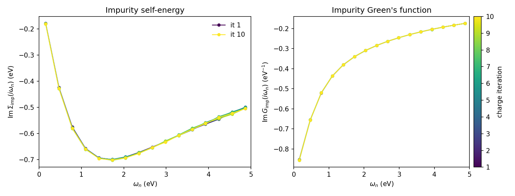
Both panels show the low-frequency Matsubara window \(0 < \omega_n < 5\) eV, with one curve per charge iteration coloured from the first (dark) to the last (light). The left panel is the imaginary part of the impurity self-energy \(\mathrm{Im}\,\Sigma_\mathrm{imp}(i\omega_n)\); its Fermi-liquid turnover — bending back towards zero as \(\omega_n \to 0\) — together with its slope near the origin (\(Z \approx 0.6\)) is the signature of the renormalized metal. The right panel is the imaginary part of the impurity Green’s function \(\mathrm{Im}\,G_\mathrm{imp}(i\omega_n)\), which stays large down to the lowest Matsubara frequency — i.e. substantial spectral weight at the Fermi level, again confirming the metallic state. The curves for all ten charge iterations lie essentially on top of each other, showing that the charge self-consistency is converged.

Note

Why track the self-energy rather than \(|G_\mathrm{imp} - G_\mathrm{loc}|\)? The latter measures the inner DMFT self-consistency (\(G_\mathrm{imp} = G_\mathrm{loc}\)), not the charge convergence of the outer loop. With a single DMFT cycle per charge update the impurity and local Green’s functions are evaluated once within the same iteration and never iterated to coincide, so their difference is dominated by the stochastic CT-SEG noise and carries no trend. The self-energy, by contrast, feels the shift of the impurity levels as the charge density is updated and converges smoothly, which is why we follow it here.