Matrix valued: 2 orbital GW self-energy of a 2D square lattice Hubbard model

%matplotlib inline
import sys, os
import numpy as np
from triqs.plot.mpl_interface import plt,oplot

from h5 import HDFArchive
from triqs.atom_diag import *

from triqs.gf import *
from triqs.operators import c, c_dag, n, dagger
from itertools import product


from triqs.lattice.tight_binding import TBLattice
from triqs.lattice.utils import k_space_path

from triqs_tprf.lattice import lattice_dyson_g0_wk, lattice_dyson_g_wk, lattice_dyson_g0_fk, dynamical_screened_interaction_W, lattice_dyson_g_fk
from triqs_tprf.gw import bubble_PI_wk, gw_sigma, lindhard_chi00, g0w_sigma

from triqs_Nevanlinna import Solver

import seaborn as sns
import scienceplots
plt.style.use(['science','notebook'])
sns.set_palette('muted')

Warning: could not identify MPI environment!

Starting serial run at: 2024-08-08 11:54:34.134002
/mnt/sw/nix/store/29h1dijh98y9ar6n8hxv78v8zz2pqfzf-python-3.11.7-view/lib/python3.11/site-packages/numpy/core/getlimits.py:549: UserWarning: The value of the smallest subnormal for <class 'numpy.float64'> type is zero.
  setattr(self, word, getattr(machar, word).flat[0])
/mnt/sw/nix/store/29h1dijh98y9ar6n8hxv78v8zz2pqfzf-python-3.11.7-view/lib/python3.11/site-packages/numpy/core/getlimits.py:89: UserWarning: The value of the smallest subnormal for <class 'numpy.float64'> type is zero.
  return self._float_to_str(self.smallest_subnormal)
/mnt/sw/nix/store/29h1dijh98y9ar6n8hxv78v8zz2pqfzf-python-3.11.7-view/lib/python3.11/site-packages/numpy/core/getlimits.py:549: UserWarning: The value of the smallest subnormal for <class 'numpy.float32'> type is zero.
  setattr(self, word, getattr(machar, word).flat[0])
/mnt/sw/nix/store/29h1dijh98y9ar6n8hxv78v8zz2pqfzf-python-3.11.7-view/lib/python3.11/site-packages/numpy/core/getlimits.py:89: UserWarning: The value of the smallest subnormal for <class 'numpy.float32'> type is zero.
  return self._float_to_str(self.smallest_subnormal)

Setup simple two orbital 2D Hubbard model on square lattice

n_orb = 2

loc = np.zeros((n_orb,n_orb))
for i in range(n_orb):
    for j in range(n_orb):
        if i != 0 and i==j:
            loc[i,j] = -0.3
        if j > i or j < i:
            loc[i,j] = -0.5

t = -1.0 * np.eye(n_orb)   #nearest neighbor hopping
tp = 0.1 * np.eye(n_orb)    #next nearest neighbor hopping

hop= {  (0,0)  :  loc,
        (1,0)  :  t,
        (-1,0) :  t,
        (0,1)  :  t,
        (0,-1) :  t,
        (1,1)  :  tp,
        (-1,-1):  tp,
        (1,-1) :  tp,
        (-1,1) :  tp}

TB = TBLattice(units = [(1, 0, 0) , (0, 1, 0)], hoppings = hop, orbital_positions= [(0., 0., 0.)]*n_orb)

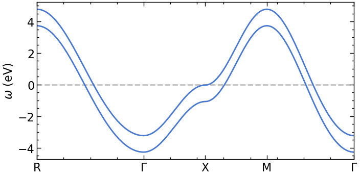
plot dispersion along high-symmetry lines

n_pts = 101
G = np.array([ 0.00,  0.00,  0.00])
M = np.array([0.5, 0.5, 0.0])
X = np.array([0.5, 0.0, 0.0])
R = np.array([0.5, 0.5, 0.5])
paths = [(R, G), (G, X), (X, M), (M, G)]

kvecs, k, ticks  = k_space_path(paths, num=n_pts, bz=TB.bz)

e_mat = TB.fourier(kvecs)
e_val = TB.dispersion(kvecs)
eps_k = {'k': k, 'K': ticks, 'eval': e_val, 'emat' : e_mat}

fig, ax = plt.subplots(1,1, figsize=(8,4), dpi=100, squeeze=False)
ax = ax.reshape(-1)

for band in range(eps_k['eval'].shape[1]):
    ax[0].plot(eps_k['k'], eps_k['eval'][:,band].real, color='C0', zorder=2.5)

ax[0].axhline(y=0,zorder=2,color='gray',alpha=0.5,ls='--')
ax[0].set_xticks(eps_k['K'])
ax[0].set_xticklabels([r'R', '$\Gamma$', 'X', 'M', r'$\Gamma$'])
ax[0].set_xlim([eps_k['K'].min(), eps_k['K'].max()])
ax[0].set_ylabel(r'$\omega$ (eV)')

plt.show()

GW in imaginary time

k_grid = (30,30,1)
k_mesh = TB.get_kmesh(n_k = k_grid)
e_k = TB.fourier(k_mesh)
eps_k = TB.dispersion(k_mesh)
mu = 0.

beta = 10
n_iw = 400
iw_mesh = MeshImFreq(beta=beta, S='Fermion', n_max=n_iw)
G0_iwk = lattice_dyson_g0_wk(mu=mu, e_k=e_k, mesh=iw_mesh)

setup bare interaction

def construct_U_kan(n_orb, U, J, Up=None, Jc=None):

    orb_range = range(0, n_orb)
    U_kan = np.zeros((n_orb, n_orb, n_orb, n_orb))

    if not Up:
        Up = U-2*J
    if not Jc:
        Jc = J

    for i,j,k,l in product(orb_range, orb_range, orb_range, orb_range):
        if i == j == k == l: # Uiiii
            U_kan[i, j, k, l] = U
        elif i == k and j == l: # Uijij
            U_kan[i, j, k, l] = Up
        elif i == l and j == k: # Uijji
            U_kan[i, j, k, l] = J
        elif i == j and k ==l: # Uiijj
            U_kan[i, j, k, l] = Jc
    return U_kan

U=1
Up=0.2
J=0.4
V_k = Gf(mesh=k_mesh, target_shape=[n_orb*1]*4)

V_bare = np.zeros((n_orb,n_orb,n_orb,n_orb))
# simple onsite intra orbital Coulomb repulsion
for i in range(n_orb):
    for j in range(n_orb):
        if i == j:
            V_bare[i,i,j,j] = U
        else:
            V_bare[i,i,j,j] = Up

V_bare = construct_U_kan(n_orb=n_orb,U=U,J=J,Up=Up)


V_k.data[:] = V_bare

Run one GW loop

print('--> pi_bubble')
PI_iwk = bubble_PI_wk(G0_iwk)

print('--> screened_interaction_W')
Wr_iwk = dynamical_screened_interaction_W(PI_iwk, V_k)

print('--> gw_self_energy')
Σ_iwk = gw_sigma(Wr_iwk, G0_iwk)

print('--> lattice_dyson_g_wk')
G_wk = lattice_dyson_g_wk(mu, e_k, Σ_iwk)

Σ_Γ_iw = Σ_iwk[:, Idx(0,0,0)]
Σ_X_iw = Σ_iwk[:, Idx(k_grid[1]-1,0,0)]

--> pi_bubble
--> screened_interaction_W
--> gw_self_energy
--> lattice_dyson_g_wk

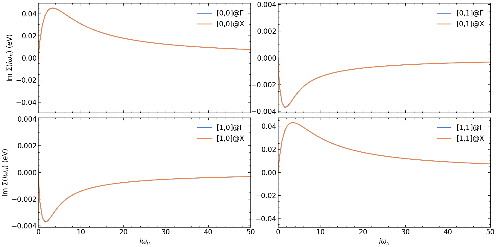
Plot results

fig, ax = plt.subplots(n_orb, n_orb, figsize=(8*n_orb,4*n_orb), dpi=100, squeeze=False,sharex=True)

shp = Σ_Γ_iw.target_shape
for i in range(n_orb):
    for j in range(n_orb):
        ax[i,j].oplot(Σ_Γ_iw[i,j].imag, label=f'[{i},{j}]@$\Gamma$')
        ax[i,j].oplot(Σ_X_iw[i,j].imag, label=f'[{i},{j}]@X')

        ax[i,j].set_xlim(0,50)

        if i == shp[0]-1:
            ax[i,j].set_xlabel(r'$i\omega_n$')
        else:
            ax[i,j].set_xlabel(r'')
        if j == 0:
            ax[i,j].set_ylabel(r'Im $\Sigma (i\omega_n)$ (eV)')
        else:
            ax[i,j].set_ylabel(r'')

plt.tight_layout(pad=0.4, w_pad=0.1, h_pad=0.4)
plt.show()

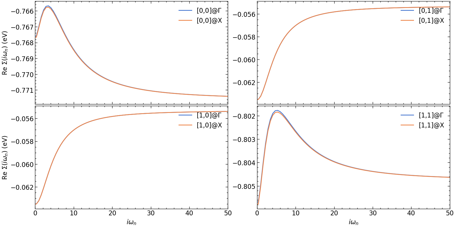
fig, ax = plt.subplots(n_orb, n_orb, figsize=(8*n_orb,4*n_orb), dpi=100, squeeze=False,sharex=True)

for i in range(n_orb):
    for j in range(n_orb):
        ax[i,j].oplot(Σ_Γ_iw[i,j].real, label=f'[{i},{j}]@$\Gamma$')
        ax[i,j].oplot(Σ_X_iw[i,j].real, label=f'[{i},{j}]@X')

        ax[i,j].set_xlim(0,50)

        if i == shp[0]-1:
            ax[i,j].set_xlabel(r'$i\omega_n$')
        else:
            ax[i,j].set_xlabel(r'')
        if j == 0:
            ax[i,j].set_ylabel(r'Re $\Sigma (i\omega_n)$ (eV)')
        else:
            ax[i,j].set_ylabel(r'')

plt.tight_layout(pad=0.4, w_pad=0.1, h_pad=0.4)
plt.show()

GW on real frequency axis

# make sure 0 is not in the mesh! Divergence for q=[0,0,0]
# no large freq mesh is needed. kmesh critical for convergence here
n_w = 100
delta = 0.1
GW_window = (-15, 15)
w_mesh = MeshReFreq(window=GW_window, n_w=n_w)


G0_wk = lattice_dyson_g0_fk(mu=mu, e_k=e_k, mesh=w_mesh, delta=delta)

print('--> pi_bubble')
PI_wk = lindhard_chi00(e_k=e_k, mesh=w_mesh, beta=beta, mu=mu, delta=delta)

print('--> screened_interaction_W')
Wr_wk = dynamical_screened_interaction_W(PI_wk, V_k)

print('--> gw_self_energy')
Σ_wk = g0w_sigma(mu=mu, beta=beta, e_k=e_k, W_fk=Wr_wk, v_k=V_k, delta=delta)

print('--> lattice_dyson_g_wk')
g_fk = lattice_dyson_g_fk(mu, e_k, Σ_wk, delta)

Σ_Γ_w = Σ_wk[:, Idx(0,0,0)]
Σ_X_w = Σ_wk[:, Idx(k_grid[1]-1,0,0)]

--> pi_bubble
--> screened_interaction_W
--> gw_self_energy
--> lattice_dyson_g_wk

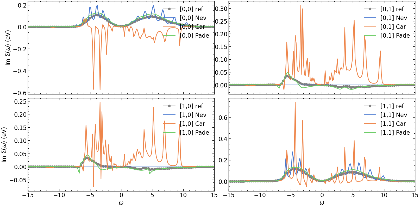
Analytic continuation

Nevanlinna

# setup Nevanlinna kernel solver
solver = Solver(kernel="CARATHEODORY")

solver.solve(Σ_Γ_iw-Σ_Γ_iw(Σ_Γ_iw.mesh.last_index()))

Σ_w_mesh = MeshReFreq(window=GW_window, n_w=n_w*2)
Σ_Γ_w_CN = solver.evaluate(Σ_w_mesh, delta)

# setup Nevanlinna kernel solver
solver = Solver(kernel="NEVANLINNA")

solver.solve(Σ_Γ_iw)

Σ_w_mesh = MeshReFreq(window=GW_window, n_w=n_w*2)
Σ_Γ_w_N = solver.evaluate(Σ_w_mesh, delta)

This is Nevanlinna analytical continuation. All off-diagonal elements will be ignored.

Pade

Σ_Γ_w_P = Σ_Γ_w_N.copy()

Σ_Γ_w_P.set_from_pade(Σ_Γ_iw, n_points=n_iw, freq_offset=delta)

Comparison

fig, ax = plt.subplots(n_orb, n_orb, figsize=(8*n_orb,4*n_orb), dpi=100, squeeze=False,sharex=True)

shp = Σ_Γ_w.target_shape
for i in range(n_orb):
    for j in range(n_orb):
        # plotting results
        ax[i,j].oplot(Σ_Γ_w[i,j].imag, '-o', c='gray', label=f'[{i},{j}] ref')
        ax[i,j].oplot(Σ_Γ_w_N[i,j].imag, label=f'[{i},{j}] Nev')
        ax[i,j].oplot(Σ_Γ_w_CN[i,j].imag, label=f'[{i},{j}] Car')
        ax[i,j].oplot(Σ_Γ_w_P[i,j].imag, label=f'[{i},{j}] Pade')


        ax[i,j].set_xlim(GW_window)
        if i == shp[0]-1:
            ax[i,j].set_xlabel(r'$\omega$')
        else:
            ax[i,j].set_xlabel(r'')
        if j == 0:
            ax[i,j].set_ylabel(r'Im $\Sigma (\omega)$ (eV)')
        else:
            ax[i,j].set_ylabel(r'')

plt.tight_layout(pad=0.4, w_pad=0.1, h_pad=0.4)
plt.show()

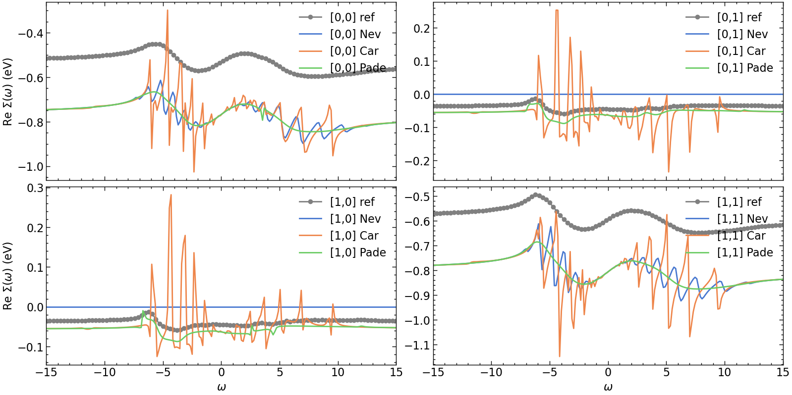
fig, ax = plt.subplots(n_orb, n_orb, figsize=(8*n_orb,4*n_orb), dpi=100, squeeze=False,sharex=True)

for i in range(n_orb):
    for j in range(n_orb):
        # plotting results
        ax[i,j].oplot(Σ_Γ_w[i,j].real, '-o', c='gray', label=f'[{i},{j}] ref')
        ax[i,j].oplot(Σ_Γ_w_N[i,j].real, label=f'[{i},{j}] Nev')
        ax[i,j].oplot((Σ_Γ_w_CN[i,j]+Σ_Γ_iw(Σ_Γ_iw.mesh.last_index())[i,j]).real, label=f'[{i},{j}] Car')
        ax[i,j].oplot(Σ_Γ_w_P[i,j].real, label=f'[{i},{j}] Pade')

        ax[i,j].set_xlim(GW_window)
        if i == shp[0]-1:
            ax[i,j].set_xlabel(r'$\omega$')
        else:
            ax[i,j].set_xlabel(r'')
        if j == 0:
            ax[i,j].set_ylabel(r'Re $\Sigma (\omega)$ (eV)')
        else:
            ax[i,j].set_ylabel(r'')

plt.tight_layout(pad=0.4, w_pad=0.1, h_pad=0.4)
plt.show()