Anderson impurity model (SIAM)

To illustrate how the NRG solver works in practice, we show the example of one-orbital Anderson impurity embedded in a flat (Wilson) conduction bath. The interacting part of the local Hamiltonian of this problem is simply:

\[\mathcal{H}_\mathrm{int} = U n_\uparrow n_\downarrow,\]

and the non-interacting Green’s function is:

\[G^{-1}_{0,\sigma} (\omega) = \omega - \epsilon_f - V^2 g(\omega).\]

In this example, there is a Coulomb interaction \(U\) on the impurity level, which is at an energy \(\epsilon_f\). The bath Green’s function is \(g(\omega)\), and it has a flat density of states over the interval \([-1,1]\). Finally, \(V\) is the hybridization amplitude between the impurity and the bath. Let us solve this problem with the NRG solver. Here is the python script:

from nrgljubljana_interface import Solver, Flat
from h5 import *

# Parameters
D, V, U = 1.0, 0.25, 1.0
e_f = -U/2.0 # particle-hole symmetric case
T = 1e-5

# Set up the Solver
S = Solver(model = "SIAM", symtype = "QS", mesh_max = 2.0, mesh_min = 1e-5, mesh_ratio = 1.01)

# Solve Parameters
sp = { "T": T, "Lambda": 2.0, "Nz": 4, "Tmin": 1e-6, "keep": 2000, "keepenergy": 10.0, "bandrescale": 1.0 }

# Model Parameters
mp = { "U1": U, "eps1": e_f }
sp["model_parameters"] = mp

# Initialize hybridization function
S.Delta_w['imp'] << V**2 * Flat(D)

# Solve the impurity model
S.solve(**sp)

# Store the Result
with HDFArchive("aim_solution.h5", 'w') as arch:
    arch["A_w"] = S.A_w
    arch["G_w"] = S.G_w
    arch["F_w"] = S.F_w
    arch["Sigma_w"] = S.Sigma_w
    arch["expv"] = S.expv

print("<n>=", S.expv["n_d"])

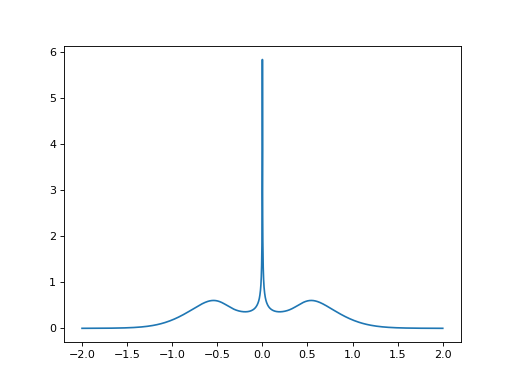
Running this script takes a few minutes and generates an HDF5 archive file called aim_solution.h5. This file contains the impurity spectral function, Green’s function, auxiliary Green’s function, self-energy, and expectation values of local variables, here \(\langle n \rangle\) and \(\langle n^2 \rangle\). Let us plot the spectral function:

import numpy as np
import matplotlib as mpl
import matplotlib.pyplot as plt

from triqs.gf import *
from h5 import *
from nrgljubljana_interface import MeshReFreqPts

def A_to_nparrays(A):
    lx = np.array(list(A.mesh.values()))
    ly = A[0,0].data.real
    return lx, ly

with HDFArchive('aim_solution.h5','r') as ar:
    # Expectation values
    print("<n>=",ar['expv']['n_d'])
    print("<n^2>=",ar['expv']['n_d^2'])

    # Spectral function
    A_w = ar['A_w']['imp']
    lx, ly = A_to_nparrays(A_w)
    plt.plot(lx, ly)
    plt.show()

As expected, the result shows a particle-hole symmetric impurity spectral function.

Let us now go through the script in some more detail:

from nrgljubljana_interface import Solver, Flat
from h5 import *

These lines import the classes to run the NRG solver and to store the results in a HDF5 archive file.

D, V, U = 1.0, 0.25, 1.0
e_f = -U/2.0 # particle-hole symmetric case
T = 1e-5

These lines define the impurity parameters, the (half)bandwidth \(D=1\), and the physical temperature \(T\).

S = Solver(model = "SIAM", symtype = "QS", mesh_max = 2.0, mesh_min = 1e-5, mesh_ratio = 1.01)

Here we construct the Solver object. The most important parameters here are the model name and its symmetry type, as well as the mesh parameters which define the logarithmic discretization mesh on which all quantities (input and output) are defined. The models are described in template files in the directory templates/. The program will automatically determine the correct block structure of hybridisation and Green’s functions from the templates. This ensures that all quantities within Solver are correctly initialized, and in particular that the block structure of all Green’s function objects is consistent.

sp = { "T": T, "Lambda": 2.0, "Nz": 4, "Tmin": 1e-6, "keep": 2000, "keepenergy": 10.0, "bandrescale": 1.0 }

This line defines, in addition to the physical temperature, the key solve parameters which affect the quality of the results: the discretization parameter \(\Lambda\), the number of the interleaved discretization meshes \(N_z\), the scale Tmin which defines the length of the Wilson chain (and which should be lower than the lowest physical temperature scale in the problem, in this case lower than the Kondo temperature), and the trucation settings which are determined by two parameters, the maximum number of states kept keep and the truncation energy cutoff keepenergy. We also explicitly set the NRG energy window to the interval \([-1:1]\), since the default is to use an energy window with the same extent as the logarithmic mesh, which in this example would be \([-2:2]\), i.e., larger than the support of the hybridisation function that we actually use; this is achieved by setting the parameter bandrescale (back) to 1. All other parameters have suitable default values for our purposes.

Finally, we have set the model parameters. These are contained in a separate Python dictionary:

mp = { "U1": U, "eps1": e_f }
sp["model_parameters"] = mp

The hybridisation function is set by the following line:

S.Delta_w['imp'] << V**2 * Flat(D)

We can now call the solver…

S.solve(**sp)

… and store the results in an HDF5 archive:

with HDFArchive("aim_solution.h5", 'w') as arch:
    arch["A_w"] = S.A_w
    arch["G_w"] = S.G_w
    arch["F_w"] = S.F_w
    arch["Sigma_w"] = S.Sigma_w
    arch["expv"] = S.expv

The expectation values can be accessed through the Python dictionary S.expv:

print("<n>=", S.expv["n_d"])

A version of this example can also be found in tutorial/1_AIM in the form of a Python script and a Jupyter (IPython) notebook.