Anderson-Holstein impurity model

Here we consider an impurity model with electron-phonon coupling, to wit the Anderson-Holstein impurity model. The interacting part of the local Hamiltonian of this problem is:

\[\mathcal{H}_\mathrm{int} = U n_\uparrow n_\downarrow + g (a+a^\dagger)(n-n_1) + \omega a^\dagger a,\]

and the non-interacting Green’s function is:

\[G^{-1}_{0,\sigma} (\omega) = \omega - \epsilon_f - V^2 g(\omega).\]

The new element (compared to the Anderson impurity model) is the presence of a phonon mode with frequency \(\omega\), which couples through e-ph coupling strength \(g\). Finally, \(n_1\) is a shift, typically either 0, 1 or \(\langle n \rangle\).

Here is the python script:

from nrgljubljana_interface import Solver, Flat
from h5 import *

# Parameters
D, V, U = 1.0, 0.2, 0    # Zero e-e interaction
e_f = -U/2.0             # particle-hole symmetric case
T = 1e-5
omega = 0.2              # phonon frequency
g1 = 0.2                 # electron-phonon coupling strength
n1 = 1                   # n1 in g1*(a+a^dag)*(n-n1)

# Set up the Solver
S = Solver(model = "Holstein/Nph=10", symtype = "QS", mesh_max = 2.0, mesh_min = 1e-5, mesh_ratio = 1.01)

# Solve Parameters
sp = { "T": T, "Lambda": 2.0, "Nz": 4, "Tmin": 1e-6, "keep": 1000, "keepenergy": 10.0, "bandrescale": 1.0 }

# Model Parameters
mp = { "U1": U, "eps1": e_f, "omega": omega, "g1": g1, "n1": n1 }
sp["model_parameters"] = mp

# Initialize hybridization function
S.Delta_w['imp'] << V**2 * Flat(D)

# Solve the impurity model
S.solve(**sp)

# Store the Result
with HDFArchive("holstein_solution.h5", 'w') as arch:
    arch["A_w"] = S.A_w
    arch["G_w"] = S.G_w
    arch["F_w"] = S.F_w
    arch["Sigma_w"] = S.Sigma_w
    arch["expv"] = S.expv

print("<n>=", S.expv["n_d"])           # occupancy
print("<nph>=", S.expv["nph"])         # average phonon number
print("<displ^2>=", S.expv["displ^2"]) # oscillator displacement squared

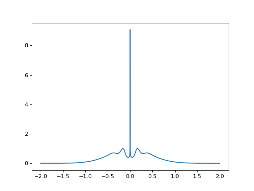
Running this script takes a few minutes and generates an HDF5 archive file called holstein_solution.h5. Let us plot the spectral function:

import numpy as np
import matplotlib as mpl
import matplotlib.pyplot as plt

from triqs.gf import *
from h5 import *
from nrgljubljana_interface import MeshReFreqPts

def A_to_nparrays(A):
    lx = np.array(list(A.mesh.values()))
    ly = A[0,0].data.real
    return lx, ly

with HDFArchive('holstein_solution.h5','r') as ar:
    A_w = ar['A_w']['imp']     # Spectral function
    lx, ly = A_to_nparrays(A_w)
    plt.plot(lx, ly)
    plt.show()

As expected, the result shows a particle-hole symmetric impurity spectral function with a (charge) Kondo resonance and side peaks at multiples of the phonon frequency \(\omega\);

Let us now go through the script in some more detail, focusing on the differences with respect to the standard Anderson impurity model.

D, V, U = 1.0, 0.2, 0    # Zero e-e interaction
e_f = -U/2.0             # particle-hole symmetric case
T = 1e-5
omega = 0.2              # phonon frequency
g1 = 0.2                 # electron-phonon coupling strength
n1 = 1                   # n1 in g1*(a+a^dag)*(n-n1)

Here we set the parameters. Note that we have set the Hubbard parameter to zero, thus this is a pure Holstein impurity problem, with the correlation effects stemming solely from the electron-phonon coupling. We set \(n_1\) to 1, to ensure particle-hole symmetry.

S = Solver(model = "Holstein/Nph=10", symtype = "QS", mesh_max = 2.0, mesh_min = 1e-5, mesh_ratio = 1.01)

Here we construct the Solver object. Note the model name which contains the phonon number cutoff (10). In NRGLjubljana_interface, the model names are actually paths to template files (either those bundled with the interface in the directory templates/, or custom templates created by the user). In the case of the Anderson-Holstein model, the template files need to be generated for a specific value of the phonon cutoff.

print("<n>=", S.expv["n_d"])           # occupancy
print("<nph>=", S.expv["nph"])         # average phonon number
print("<displ^2>=", S.expv["displ^2"]) # oscillator displacement squared

The Anderson-Holstein model defines several additional expectation values pertaining to the phonon degree of freedom.