Random number generators

It is possible (and highly recommended!) to use different random number generators with the CTQMC solver. A list of available random generators can be obtained with:

from triqs.random_generator import *
print random_generator_names_list()

The names in this list can then be used to set the random_name keyword argument in the solve() method of the CTQMC solver. Here is an example where the same run is done twice, but using different random generators.

from triqs.gf import *
from triqs.operators import *
from h5 import HDFArchive
from triqs_cthyb import Solver
import triqs.utility.mpi as mpi

D, V, U = 1.0, 0.2, 4.0
e_f, beta = -U/2.0, 50

# Construct the impurity solver
S = Solver(beta = beta, gf_struct = [ ('up',1), ('down',1) ])

# Loop for two random generators
for random_name in ['mt11213b','lagged_fibonacci607']:

    for spin, g0 in S.G0_iw:
        g0 << inverse(iOmega_n - e_f - V**2 * Wilson(D))

    # Solve using random_name as a generator
    S.solve(h_int = U * n('up',0) * n('down',0),   # Local Hamiltonian
            n_cycles = 100000,                     # Number of QMC cycles
            length_cycle = 200,                    # Length of one cycle
            n_warmup_cycles = 10000,               # Number of warmup cycles
            random_name = random_name)             # Name of the random generator

    # Save the results in an hdf5 file (only on the master node)
    if mpi.is_master_node():
        with HDFArchive("random.h5") as Results:
            Results["G_iw%s"%(random_name)] = S.G_iw

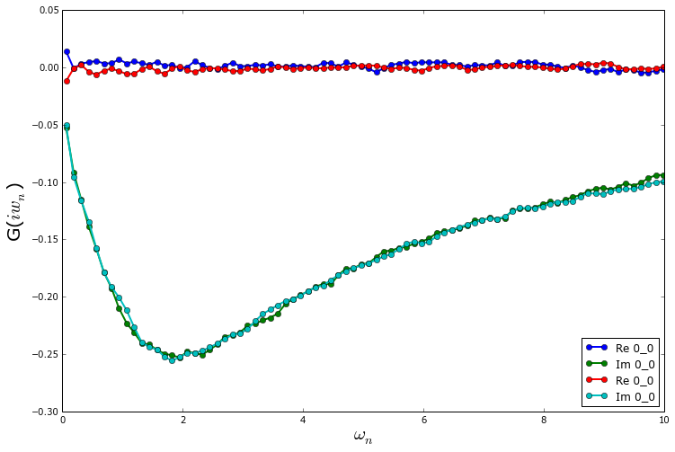
The resulting Green’s functions are:

As one can see from the plots, the two random number generators lead to very similar results. On these short runs, one also notices that more statistics will be needed to have a reliable Green’s function at low frequencies.