Tail fitting via the CRM Dyson solver

Computing the self-energy within DMFT is a numerically unstable problem that leads to large errors at high-frequencies. These errors must be corrected in order to update the local Green’s function for the next DMFT cycle. Historically, the high-frequency error in the self-energy has been dealt with by fitting a high-frequency expansion of the self-energy to the raw QMC data (this procedure is referred to as tail fitting). However, tail fitting is cumbersome and error prone. Morevoer, it requires ‘by-hand’ tuning by the user. Recently, a new algorithm has been developed to address the tail fitting problem by recasting the solution of the numerically unstable Dyson equation as a constrained minimization problem (CRM). For more complete details of the algorithm and examples, please see arXiv:2310.01266 and this TRIQS/cthyb tutorial.

In the this tutorial, we will demonstrate how to use the CRM method to compute the self-energy from the TRIQS/cthyb impurity solver for a simple one-orbital Bethe lattice problem. Experts will note that for this specific problem, the self-energy is not needed to update the Green’s function in the DMFT loop but remains sufficient for illustrative purposes.

Setup

First we setup a simple Bethe lattice impurity model. Here we use the delta_interface=True of the solver, compared to other tutorials with the Bethe lattice. The below cells demonstrate how one can set up the impurity Green’s function, hybridization function, and run the solver.

from h5 import HDFArchive
from triqs.gf import Gf, iOmega_n, make_gf_from_fourier, make_zero_tail, fit_hermitian_tail, inverse
from triqs.operators import c, c_dag, n
from triqs.gf.descriptors import SemiCircular
from itertools import product

# plotting interface
from triqs.plot.mpl_interface import plt, oplot

from triqs_cthyb.solver import Solver

Warning: could not identify MPI environment!

Starting serial run at: 2024-06-12 13:42:54.707417

# Set up a few parameters
U = 4.0
half_bandwidth = 1.0
chemical_potential = U/2.0
beta = 10
n_cycles = int(1e+6)
length_cycle = 50
warmup = int(1e+5)

# we are using the delta_interface here compared to earlier examples!
S = Solver(beta = beta, gf_struct = [ ('up',1), ('down',1) ], delta_interface=True, n_iw=501, n_tau=5001)


# Initalize the Green's function to a semi circular DOS
S.G_iw << SemiCircular(half_bandwidth)
delta_iw = S.G_iw.copy()
delta_iw.mesh.set_tail_fit_parameters(tail_fraction=0.5, n_tail_max=40, expansion_order=2)

# first moment of delta is 0
known_moments = make_zero_tail(delta_iw['up'], 1)

# prepare non-interacting impurity Hamiltonian
N = sum(n(sp,orb) for sp, orb in [('up', 0), ('down', 0)])
h_loc0 = -chemical_potential*N

# Now do the DMFT loop once
# Compute new S.G0_iw with the self-consistency condition while imposing paramagnetism
g_sym = 0.5 * ( S.G_iw['up'] + S.G_iw['down'] )

G0_iw = S.G_iw['up'].copy()
G0_iw << inverse(iOmega_n + chemical_potential - (half_bandwidth/2.0)**2 * g_sym)

for name, delta in delta_iw:
    delta << (half_bandwidth/2.0)**2 * g_sym

    tail, err = fit_hermitian_tail(delta, known_moments)
    S.Delta_tau[name] << make_gf_from_fourier(delta, S.Delta_tau.mesh, tail).real

# Run the solver without any tail-fitting or legendre measurements
S.solve(h_int = U * n('up',0) * n('down',0),    # Local Hamiltonian
        n_cycles = n_cycles,                    # Number of QMC cycles
        length_cycle = length_cycle,            # Length of a cycle
        n_warmup_cycles = warmup,               # How many warmup cycles
        h_loc0 = h_loc0,                        # non-interacting impurity Hamiltonian
        measure_density_matrix = True,          # measure impurity density matrix for moments
        use_norm_as_weight = True)

print('imp occ: {:2.4f}'.format(S.G_iw.total_density().real))

╔╦╗╦═╗╦╔═╗ ╔═╗  ┌─┐┌┬┐┬ ┬┬ ┬┌┐
 ║ ╠╦╝║║═╬╗╚═╗  │   │ ├─┤└┬┘├┴┐
 ╩ ╩╚═╩╚═╝╚╚═╝  └─┘ ┴ ┴ ┴ ┴ └─┘

The local Hamiltonian of the problem:
-2*c_dag('down',0)*c('down',0) + -2*c_dag('up',0)*c('up',0) + 4*c_dag('down',0)*c_dag('up',0)*c('up',0)*c('down',0)
Using autopartition algorithm to partition the local Hilbert space
Found 4 subspaces.

Warming up ...
13:42:55   2% ETA 00:00:04 cycle 2017 of 100000
13:42:57  47% ETA 00:00:02 cycle 47928 of 100000
13:42:59 100% ETA 00:00:00 cycle 99999 of 100000



Accumulating ...
13:42:59   0% ETA 00:00:45 cycle 2195 of 1000000
13:43:01   4% ETA 00:00:43 cycle 46241 of 1000000
13:43:04  10% ETA 00:00:41 cycle 101455 of 1000000
13:43:07  17% ETA 00:00:38 cycle 170514 of 1000000
13:43:11  25% ETA 00:00:34 cycle 256794 of 1000000
13:43:16  36% ETA 00:00:29 cycle 364557 of 1000000
13:43:22  49% ETA 00:00:23 cycle 498855 of 1000000
13:43:30  66% ETA 00:00:15 cycle 666798 of 1000000
13:43:39  87% ETA 00:00:05 cycle 876758 of 1000000
13:43:45 100% ETA 00:00:00 cycle 999999 of 1000000


[Rank 0] Collect results: Waiting for all mpi-threads to finish accumulating...
[Rank 0] Timings for all measures:
Measure                                    | seconds
Auto-correlation time                      | 0.300902
Average order                              | 0.0362441
Average sign                               | 0.0312844
Density Matrix for local static observable | 1.01593
G_tau measure                              | 0.112968
Total measure time                         | 1.49733
[Rank 0] Acceptance rate for all moves:
Move set Insert two operators: 0.141738
  Move  Insert Delta_up: 0.141697
  Move  Insert Delta_down: 0.141778
Move set Remove two operators: 0.141941
  Move  Remove Delta_up: 0.141938
  Move  Remove Delta_down: 0.141944
Move set Insert four operators: 0.0360915
  Move  Insert Delta_up_up: 0.0212035
  Move  Insert Delta_up_down: 0.0508802
  Move  Insert Delta_down_up: 0.0510066
  Move  Insert Delta_down_down: 0.0212639
Move set Remove four operators: 0.0359989
  Move  Remove Delta_up_up: 0.0209461
  Move  Remove Delta_up_down: 0.0508458
  Move  Remove Delta_down_up: 0.0511521
  Move  Remove Delta_down_down: 0.021033
Move  Shift one operator: 0.212673
[Rank 0] Warmup lasted: 4.42282 seconds [00:00:04]
[Rank 0] Simulation lasted: 45.9534 seconds [00:00:45]
[Rank 0] Number of measures: 1000000
Total number of measures: 1000000
Average sign: 1
Average order: 1.98421
Auto-correlation time: 0.852318
imp occ: 0.9877

Warning :: Trace of the density matrix is 1.000000000001 instead of 1

First, we will compute the self-energy by direct inversion from the Dyson equation.

# average impurity Green's function:
G_iw_avg = 0.5*(S.G_iw['up']+S.G_iw['down'])
G_tau_avg = 0.5*(S.G_tau['up']+S.G_tau['down'])

# calculate Sigma via standard Dyson equation:
S_iw_dyson = inverse(G0_iw) - inverse(G_iw_avg)

Plot the resulting self-energy:

fig, ax = plt.subplots(2,1,dpi=200,figsize=(6,6),sharex=True)
ax = ax.reshape(-1)
fig.subplots_adjust(wspace=0.2, hspace=0.08)


ax[0].oplot(S_iw_dyson.real, '-o', label='Dyson')
ax[1].oplot(S_iw_dyson.imag, '-o', label='Dyson')

ax[0].set_xlim(0,40)
ax[0].set_ylim(1.6,2.4)
ax[1].set_ylim(-2.5,0.2)
ax[0].set_ylabel(r'Re $\Sigma_\mathrm{imp}$ (eV)')
ax[1].set_ylabel(r'Im $\Sigma_\mathrm{imp}$ (eV)')
ax[0].set_xlabel(r'')
ax[1].set_xlabel(r'$i \omega_n$')

plt.show()

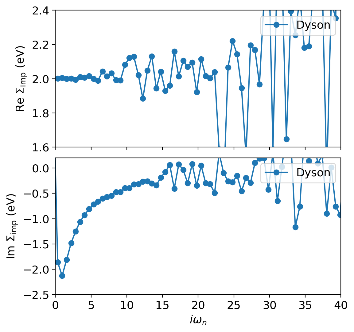
One can immediately observe a numerical catastrophe occurs at high-frequencies (which is due to the instability of the Dyson equation). The goal is to “repair” the noisy tail of the self-energy, such that it can be used in the subsequent DMFT update.

Using the Constrained Residual Minimization Dyson solver

The CRM algorithm (arXiv:2310.01266) introduces a novel method for computing the self-energy, effectively bypassing the numerical instability associated with directly inverting the Dyson equation. This is achieved by representing all quantities in a compact basis. We use the discrete Lehmann representation (DLR) to do this. For more details on the DLR, please see Phys. Rev B 105, 235115 (2022). With all quantities represented in this basis, one can construct a constrained minimization problem for the self-energy, where the constraints are its first two moments of its high-frequency expansion. These moments can be directly measured to high accuracy by the CT-HYB impurity solver.

We begin by constructing the DLR basis. The DLR basis is built by specifying two parameters \(\omega_{\mathrm{max}}\) and \(\varepsilon\). The first parameter (\(\omega_{\mathrm{max}}\)) is physically meaningful and corresponds to the spectral width of the impurity problem that you are studying. The second parameter \(\varepsilon\) represenst the accuracy of the DLR basis to represent any spectral representable Green’s function with the given \(\omega_{\mathrm{max}}\), and can be thought of as an error tolerance. In this tutorial, we will set \(\omega_{\mathrm{max}} = 2.5\) eV and \(\varepsilon = 10^{-7}\). As an exercise, one can play with these parameters and observe how the resulting self-energies change.

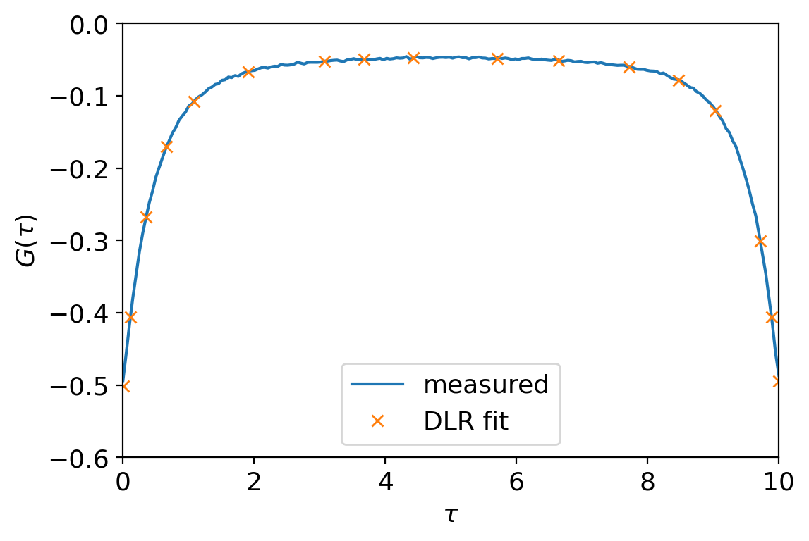
We start by fitting a DLR Green’s function to our imaginary time Green’s function using the TRIQS function fit_gf_dlr. In the figure below, we see the DLR Green’s function (orange crosses) gives a compact representation of the full imaginary time Green’s function (solid blue line).

from triqs.gf import fit_gf_dlr, make_gf_dlr_imtime

G_dlr_imp = fit_gf_dlr(G_tau_avg, w_max = 3, eps = 1e-7)

fig, ax = plt.subplots(1,dpi=200,figsize=(6,4),sharex=True)

# plot rebinned G_tau to suppress noise slightly for plotting
ax.oplot(G_tau_avg.rebinning_tau(200).real, '-', label='measured')
ax.oplot(make_gf_dlr_imtime(G_dlr_imp).real, label='DLR fit')

ax.set_xlim(0,beta)
ax.set_ylim(-0.6,0.0)
ax.set_ylabel(r'$G(\tau)$')

ax.set_xlabel(r'$\tau$')
plt.legend(loc='lower center')
plt.show()

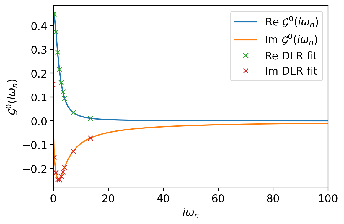
We repeat the process to obtain \(\mathcal{G}^{0}\) in the DLR basis. We can achieve this by directly reading off the values of \(\mathcal{G}^{0}(i\omega_{n})\) at the DLR nodes \(i\omega_{n_{k}}\), since \(\mathcal{G}^{0}\) is typically given without noise.

from triqs.gf import MeshDLRImFreq

# construct DLR iw empty Gf container
mesh_iw = MeshDLRImFreq(G_dlr_imp.mesh)
G0_dlr_iw = Gf(mesh=mesh_iw, target_shape=G_dlr_imp.target_shape)

# fill G0_dlr_iw from full Matsubara version
for iwn in mesh_iw:
    G0_dlr_iw[iwn] = G0_iw(iwn.value)

fig, ax = plt.subplots(1,dpi=200,figsize=(6,4),sharex=True)

ax.oplot(G0_iw.real, '-', label=r'Re $\mathcal{G}^0(i\omega_n)$')
ax.oplot(G0_iw.imag, '-', label=r'Im $\mathcal{G}^0(i\omega_n)$')
ax.oplot(G0_dlr_iw.real, label='Re DLR fit')
ax.oplot(G0_dlr_iw.imag, label='Im DLR fit')

ax.set_xlim(0,100)

ax.set_ylabel(r'$\mathcal{G}^0(i\omega_n)$')

ax.set_xlabel(r'$i \omega_n$')
plt.show()

We now have everything we need to run the CRM solver (minimize_dyson). The required inputs are a \(G\), \(\mathcal{G}^{0}\), and the high-frequency moments of the self-energy, which are stored in the Solver class as Sigma_moments. Both \(G\), \(\mathcal{G}^{0}\) have to be given on one of the DLR meshes (MeshDLR, MeshDLRImFreq, or MeshDLRImTime)

from triqs.gf.dlr_crm_dyson_solver import minimize_dyson
from triqs.gf import make_gf_imfreq

# now use the solver
S_dlr, S_HF, residual = minimize_dyson(G0_dlr = G0_dlr_iw,
                                       G_dlr = G_dlr_imp,
                                       Sigma_moments= 0.5*(S.Sigma_moments['up']+S.Sigma_moments['down'])) # average moments for higher accuracy here

# Since a spectral representable G has no constant we have to manually add the Hartree shift after the solver is finished again
S_iw_crm = make_gf_imfreq(S_dlr, n_iw=S_iw_dyson.mesh.n_iw) + S_HF

`xtol` termination condition is satisfied.
Number of iterations: 318, function evaluations: 2835, CG iterations: 141, optimality: 1.01e+01, constraint violation: 2.56e-10, execution time: 0.83 s.
`xtol` termination condition is satisfied.
L2 norm of residual (G-G₀-G₀ΣG): 5.6408e-04
Σ1 constraint diff: 2.6589e-10

The output of minimize_dyson reports if the termination of scipy minimize has been successful (scipy.optimize.OptimizeResult.message). Next the final number of iterations and other stats are reported by scipy minimize. Finally, the L2 norm of the residual is printed and the constraint violation if the second moment of Sigma is given.

fig, ax = plt.subplots(2,1,dpi=200,figsize=(6,6),sharex=True)
ax = ax.reshape(-1)
fig.subplots_adjust(wspace=0.2, hspace=0.08)


ax[0].oplot(S_iw_dyson.real, '-o', label='Dyson')
ax[1].oplot(S_iw_dyson.imag, '-o', label='Dyson')

ax[0].oplot(S_iw_crm.real, '-o', label='CRM')
ax[1].oplot(S_iw_crm.imag, '-o', label='CRM')

ax[0].set_xlim(0,40)
ax[0].set_ylim(1.5,2.5)
ax[1].set_ylim(-2.5,0.)
ax[0].set_ylabel(r'Re $\Sigma_\mathrm{imp}$ (eV)')
ax[1].set_ylabel(r'Im $\Sigma_\mathrm{imp}$ (eV)')
ax[0].set_xlabel(r'')
ax[1].set_xlabel(r'$i \omega_n$')
ax[1].legend(loc='lower right')
plt.show()

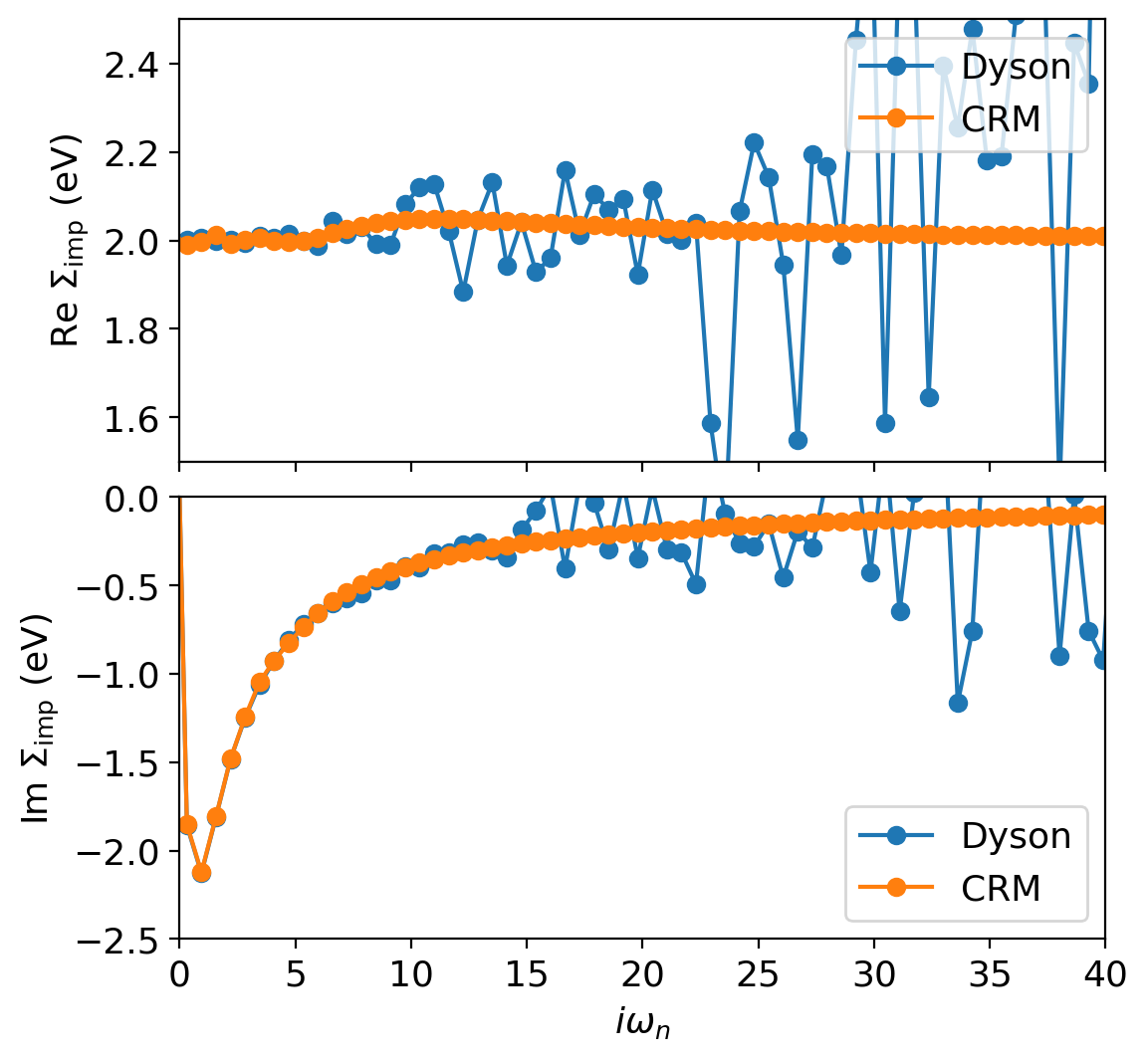
The resulting self-energy computed within the CRM scheme is absent of the high-frequency noise while maintaining the same accuracy at low-frequencies!

Important: Because the DLR requires inputs (\(\omega_{\mathrm{max}}\), \(\varepsilon\)) to determine the basis, one should check that the values of \(\omega_{\mathrm{max}}\) and \(\varepsilon\) are chosen properly. In most cases, one can leave \(\varepsilon\) fixed (\(\varepsilon\sim10^{-6}-10^{-7}\)) and converge \(\omega_{\mathrm{max}}\), which is demonstrated (and recommended) explicitly in arXiv:2310.01266.

Finally, this tutorial demonstrates some caveat of the DLR representation. The real part of \(\Sigma_{imp}\) is constant for the half-filled Bethe lattice, which is inherently hard to be represented by DLR. One always obtains in this example a slighlty oscillating solution. However, the high frequency tail is correctly preserved by the provided moments.