High Frequency Moments of the Green’s Functions and Self-energy
We present here the derivation of the high-frequency moments of the Green’s function and self-energy, as well as show case how these high frequency moments can be computed and utilized within TRIQS/cthyb.
Derivation
The following derivation follows closely Rev. Mod. Phys 83, 349 (2011) and Phys. Rev. B 84, 073104 (2011).
The high-frequency expansion of the Green’s function takes the following form
where the coefficients are related to time derivatives of the Green’s function:
where \(H\) is the Hamiltonian of the system. For the purpose of this cthyb tutorial we assume \(H\) to be the general Anderson impurity hamiltonian,
In DMFT the coefficients for the Weiss field \(\mathbf{G}_{0}\) can be obtained from the same expressions as the Green’s function with the hamiltonian replaced with only the non-interacting part.
To derive the analogous coefficients for the self-energy, we start with the Dyson equation,
Using the high-frequency expression for the Green’s function and Weiss field we obtain,
Expanding this expression for large \(i\omega_{n}\) and simplifying yields,
We now identify the leading terms,
Note, that \((\mathbf{G}_{0})_{1}\) are just the crystal field levels inside of the impurity problem \(\mathbf{E}\). We can simplify these expressions by plugging in their definitions from above,
Implentation in TRIQS/cthyb
The leading two moments of \(\mathbf{G}\) and of \(\mathbf{\Sigma}\) are automatically calculated and stored as members of the TRIQS/cthyb solver when measure_density_matrix = True. The moments for the Green’s function and self-energy are stored as Solver.G_moments and Solver.Sigma_moments, with the matching block structure of the Gf objects. Additionally, the Hartree shift \(\mathbf{\Sigma}^\infty\) is stored as Solver.Sigma_Hartree.
The moments of the Green’s function are used in the Fourier transform of \(G(\tau)\) to \(G(i\omega_{n})\) in the solver post-processing automatically if available. The moments of the self-energy are used in the tail fitting routine, where the first two known_moments now correspond to the calculated first and second moments of the self-energy.
[1]:
from triqs.gfs import *
from triqs.operators import *
from triqs_cthyb import Solver
import triqs.utility.mpi as mpi

import numpy as np
from triqs.plot.mpl_interface import plt,oplot
Warning: could not identify MPI environment!
Starting serial run at: 2023-02-02 09:38:30.738159
[2]:
D, V, U = 1.0, 0.2, 4.0

ef, beta = -U/2.0, 50
H = U*n('up',0)*n('down',0)
S = Solver(beta=beta, gf_struct=[('up',1), ('down', 1)])

for name, g0 in S.G0_iw: g0 << inverse(iOmega_n - ef - V**2 * Wilson(D))

S.solve(h_int = H,
                n_cycles =500000,
                length_cycle = 200,
                n_warmup_cycles = 100000,
                measure_density_matrix=True, # moments will be calculated automatically
                use_norm_as_weight = True,
                )
╔╦╗╦═╗╦╔═╗ ╔═╗  ┌─┐┌┬┐┬ ┬┬ ┬┌┐
 ║ ╠╦╝║║═╬╗╚═╗  │   │ ├─┤└┬┘├┴┐
 ╩ ╩╚═╩╚═╝╚╚═╝  └─┘ ┴ ┴ ┴ ┴ └─┘

The local Hamiltonian of the problem:
-2*c_dag('down',0)*c('down',0) + -2*c_dag('up',0)*c('up',0) + 4*c_dag('down',0)*c_dag('up',0)*c('up',0)*c('down',0)
Using autopartition algorithm to partition the local Hilbert space
Found 4 subspaces.

Warming up ...
09:38:33   0% ETA 00:00:15 cycle 661 of 100000
09:38:35  12% ETA 00:00:14 cycle 12541 of 100000
09:38:38  30% ETA 00:00:10 cycle 30560 of 100000
09:38:41  52% ETA 00:00:07 cycle 52654 of 100000
09:38:45  75% ETA 00:00:03 cycle 75715 of 100000


Accumulating ...
09:38:48   0% ETA 00:01:09 cycle 723 of 500000
09:38:50   3% ETA 00:01:08 cycle 15022 of 500000
09:38:53   6% ETA 00:01:05 cycle 32974 of 500000
09:38:56  11% ETA 00:01:02 cycle 55408 of 500000
09:39:00  16% ETA 00:00:58 cycle 83197 of 500000
09:39:05  23% ETA 00:00:54 cycle 117863 of 500000
09:39:11  32% ETA 00:00:48 cycle 160877 of 500000
09:39:19  43% ETA 00:00:40 cycle 215435 of 500000
09:39:29  56% ETA 00:00:31 cycle 281909 of 500000
09:39:41  71% ETA 00:00:21 cycle 355564 of 500000
09:39:56  91% ETA 00:00:06 cycle 455301 of 500000


[Rank 0] Collect results: Waiting for all mpi-threads to finish accumulating...
[Rank 0] Timings for all measures:
Measure                                    | seconds
Auto-correlation time                      | 0.144108
Average order                              | 0.0375342
Average sign                               | 0.0416869
Density Matrix for local static observable | 0.732204
G_tau measure                              | 0.0985052
Total measure time                         | 1.05404
[Rank 0] Acceptance rate for all moves:
Move set Insert two operators: 0.0448675
  Move  Insert Delta_up: 0.044915
  Move  Insert Delta_down: 0.0448199
Move set Remove two operators: 0.0448576
  Move  Remove Delta_up: 0.04491
  Move  Remove Delta_down: 0.0448052
Move set Insert four operators: 0.00347959
  Move  Insert Delta_up_up: 0.00269973
  Move  Insert Delta_up_down: 0.00431061
  Move  Insert Delta_down_up: 0.00423298
  Move  Insert Delta_down_down: 0.002676
Move set Remove four operators: 0.00348254
  Move  Remove Delta_up_up: 0.00270066
  Move  Remove Delta_up_down: 0.00431291
  Move  Remove Delta_down_up: 0.00424282
  Move  Remove Delta_down_down: 0.0026742
Move  Shift one operator: 0.0350781
[Rank 0] Warmup lasted: 15.3982 seconds [00:00:15]
[Rank 0] Simulation lasted: 74.6982 seconds [00:01:14]
[Rank 0] Number of measures: 500000
Total number of measures: 500000
Average sign: 1
Average order: 1.2027
Auto-correlation time: 0.358059
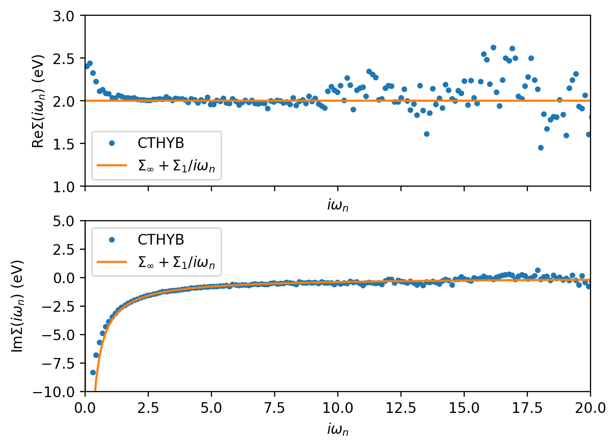
Now, we can compare the high-frequency expansion of the self-energy to the real and imaginary parts of the self-energy obtained from the Dyson equation using the sampled Green’s function and input Weiss field. Let us first have a look at the calculated moments and then plot the real part, corresponding to the overall Hartree shift, and the imaginary part of the measured self-energy together with the high-frequency expansion obtained from the moments:
[3]:
for block, moment in S.Sigma_moments.items():
    print('-------')
    print(f'{block}:')
    for i, value in enumerate(moment):
        print(f'𝚺_{i}= {value[0,0].real:1.4f}')
-------
up:
𝚺_0= 2.0033
𝚺_1= 4.0000
-------
down:
𝚺_0= 1.9967
𝚺_1= 4.0000
[4]:
for block, moment in S.G_moments.items():
    print('-------')
    print(f'{block}:')
    for i, value in enumerate(moment):
        print(f'Gimp_{i}= {value[0,0].real:1.4f}')
-------
up:
Gimp_0= 0.0000
Gimp_1= 1.0000
Gimp_2= 0.0033
-------
down:
Gimp_0= 0.0000
Gimp_1= 1.0000
Gimp_2= -0.0033
[5]:
fig, ax = plt.subplots(2,1, sharex=True, dpi=200)

# prepare highfreq expansion for plotting on grid
iwn = np.array([complex(x) for x in S.Sigma_iw.mesh])
high_freq = S.Sigma_moments['up'][0][0,0] + S.Sigma_moments['up'][1][0,0]/iwn

# plot Re component
ax[0].oplot(S.Sigma_iw['up'][0,0].real, 'o', ms=3, label='CTHYB')
ax[0].plot(iwn.imag, high_freq.real, '-', label=r'$\Sigma_{\infty} + \Sigma_{1}/i\omega_{n}$')

# plot Im component
ax[1].oplot(S.Sigma_iw['up'][0,0].imag, 'o', ms=3, label='CTHYB')
ax[1].plot(iwn.imag, high_freq.imag, '-', label=r'$\Sigma_{\infty} + \Sigma_{1}/i\omega_{n}$')

ax[0].legend(); ax[1].legend()
ax[0].set_xlabel(r'$i\omega_{n}$');
ax[1].set_xlabel(r'$i\omega_{n}$');
ax[0].set_ylabel(r'Re$\Sigma(i\omega_{n})$ (eV)')
ax[1].set_ylabel(r'Im$\Sigma(i\omega_{n})$ (eV)')
ax[0].set_xlim(0, 20);
ax[0].set_ylim(1,3); ax[1].set_ylim(-10, 5)
plt.subplots_adjust(wspace=0.5)
plt.show()
Additionally, we can verify the relationship between the first moment of the Green’s function and first moment of the self-energy,
where \(\mathbf{E}\) are the local impurity levels.
[6]:
E = {key[-1][1][0] : coef for key, coef in S.h_loc0}
print((S.Sigma_moments['up'][0]- S.G_moments['up'][-1] + E['up'])[0,0].real)
-2.3092638912203256e-14
Hence, the above equation holds exactly up to machine precision!