Convergence test of CTHYB solver parameters
Overview
The goal of this tutorial is to learn how to choose the parameters for the CTHYB solver in order to obtain accurate results with an optimized efficiency. The solver parameters investigated in this notebook are the following:
length_cycle: The number of Monte Carlo updates in a cycle, i.e. between two consecutive measurements.n_warmup_cycles: The number of warmup (thermalization) cycles at the beginning of the simulation before any measurements are made.n_cycles: The total number of QMC measurements.n_iw: The number of Matsubara frequencies used for the representation of the Green’s functions.n_l: The number of Legendre polynomials used in the accumulations of the Green’s functions.n_tau: The number of imaginary time points used for the representation of the Green’s functions.
This tutorial will help the user develop an intuition on how to perform the convergence tests for each parameter. Every test needs to be tailored according to the user’s case of study.
To run this notebook you need to import the modules below. For installation guide please refer to TRIQS and CTHYB webpages.
[1]:
import numpy as np
from math import pi
from triqs.gfs import *
from triqs.plot.mpl_interface import oplot,plt
from matplotlib import pyplot
from triqs.gfs import make_gf_from_fourier
from triqs.operators import *
from h5 import *
from h5 import HDFArchive
from triqs_cthyb import Solver
import scipy.optimize as opt
import os
import math
import matplotlib as mpl
from matplotlib.markers import MarkerStyle

# To make plots in interactive mode
%matplotlib inline

# Make all figures slightly bigger
mpl.rcParams['figure.dpi']=120
Warning: could not identify MPI environment!
Starting serial run at: 2022-09-27 11:43:09.629092
[2]:
from triqs_cthyb.version import show_version
show_version()
You are using triqs_cthyb version 3.1.0
1. length_cycle
Number of moves (or updates) between each measurement. In CTHYB, the Markov Chain is based on a sampling of the partition function. One of the measured observables in CTHYB is the Green’s function in imaginary time \(G(\tau)\). Each “move” modifies the configuration of the system (or state of the system which here is \(\mathcal{C}=d^{\dagger}_{\alpha_{1}}(\tau_1) d_{\alpha^{'}_{1}}(\tau^{'}_1) d^{\dagger}_{\alpha_{2}}(\tau_2) . . . d_{\alpha}(\tau_N)\)) by inserting/removing pairs of operators, or by moving operators in the configuration. Let’s imagine each measurement is made every L moves, then we can say that these L moves form a cycle and the length of the cycle is L.
The reason why we do not want to measure, for example \(G(\tau)\), after each move is because we want the configurations to be decorrelated from each other. To get an idea of decorrelation, we can look at the sign or expansion order which vary from one configuration to another. Plotting the standard deviation of sign/order versus the size of the data bins used to determine the error shows that it converges to a value called auto-correlation time. If,
auto-correlation time\(>\) 1 : Consecutive measurements are correlated, i.e. measurements are performed too close to one another. This is not recommended if the the measurement process is time-consuming or if the error bars need to be accurate.Length_cycleshould be increased.auto-correlation time\(\sim\) 1 : Consecutive measurements are uncorrelated often enough.Length_cycleis the correct value.auto-correlation time\(\ll\) 1 : Many more moves are performed even though the measurements would be uncorrelated. It means many less samples will be measured, requiring much longer calculation times for the same statistical noise. Moreover, it increases the error on \(G(\tau)\).Length_cycleshould be decreased.
It must be noted that auto-correlation time depends on the measured observable (i.e. sign or expansion order), therefore it should be taken with caution. Ideally auto-correlation time should be of order one. If the measurement process is fast, there is no drawback in measuring too often (auto-correlation time \(>\) 1). However there is a drawback in measuring too rarely (auto-correlation time \(\ll\) 1).
Here we take a single orbital Hubbard model at half-filling with a semi-circular density of states for three different betas \(\mathcal{\beta} = 10, 20, 30 (1/eV)\) and plot auto_correlation time vs length_cycle. The fit of a 1/x function approximately shows the converged value of length_cycle for each \(\beta\).
[ ]:
t = 1.0    # Half bandwidth
betas = [10, 20, 30]
n_loops = 1
U = 2.0
mu = 0.0
length_cycle = np.arange(20,520,20)

for b in range(len(betas)):
    if not os.path.exists('../../../data/len_cyc_b%i'%betas[b]):
        os.makedirs('../../../data/len_cyc_b%i'%betas[b])

    for j in range(len(length_cycle)):
        S = Solver(beta = betas[b], gf_struct = [('up',1), ('down',1)])
        S.G_iw << SemiCircular(2*t)
        # DMFT loop with self-consistency
        for i in range(n_loops):
            print("\n\nIteration = %i / %i" % (i+1, n_loops))
            # Symmetrize the Green's function and use self-consistency
            g = 0.5 * ( S.G_iw['up'] + S.G_iw['down'] )
            for name, g0 in S.G0_iw:
                g0 << inverse( iOmega_n + U/2.0 - mu - t**2 * g )

                # Solve the impurity problem
            S.solve(h_int = U * n('up',0) * n('down',0),     # Local Hamiltonian
                n_cycles  = 10000,                           # Number of QMC cycles
                length_cycle = length_cycle[j],              # Number of Monte Carlo moves in a cycle
                n_warmup_cycles = 3000,                      # Warmup cycles
                )
            # Save iterations in archive
            with HDFArchive('../../../data/len_cyc_b%i/half-U-lc%i.h5'%(betas[b], length_cycle[j])) as A:
                A['a%i'%i] = S.auto_corr_time
                A['b%i'%i] = S.average_order
[33]:
# Define the function for fitting a curve
def func(x, a):
     return a* 1/(x)

fig, ax = plt.subplots(1, 1, figsize=(8, 6))
marker=['-^', '-o', '-s']
for b in range(len(betas)):
    auto_corr_time = []
    for j in range(len(length_cycle)):
        R = HDFArchive('../../../data/len_cyc_b%i/half-U-lc%i.h5'%(betas[b], length_cycle[j]), 'r')
        auto_corr_time.append(R['a0'])
    optimizedParameters, pcov = opt.curve_fit(func, length_cycle, auto_corr_time);      # Fit the curve
    ax.plot(length_cycle, func(length_cycle, *optimizedParameters), color='k');
    ax.plot(length_cycle, auto_corr_time, marker[b], fillstyle="none", label='%i'%betas[b])
    ax.text(10, 0.03/(1.9**b), r'length_cycle$\sim %i$ for $\beta=%i$'%(math.ceil(optimizedParameters), betas[b]), fontsize=12)
ax.set_yscale("log")
ax.text(10, 0.08, 'Auto_correlation time will be\nequal to one at:', fontsize=12)
ax.set_ylabel('Auto-correlation time',fontsize=18)
ax.set_xlabel('length_cycle',fontsize=18)
plt.legend(title=r'$\beta(\frac{1}{eV})$', title_fontsize=16, fontsize=14)
ax.axhline(y=1, linestyle='--', color='k')
ax.text(5, 0.7, '$auto-correlation = 1$', fontsize = 10)
plt.show()
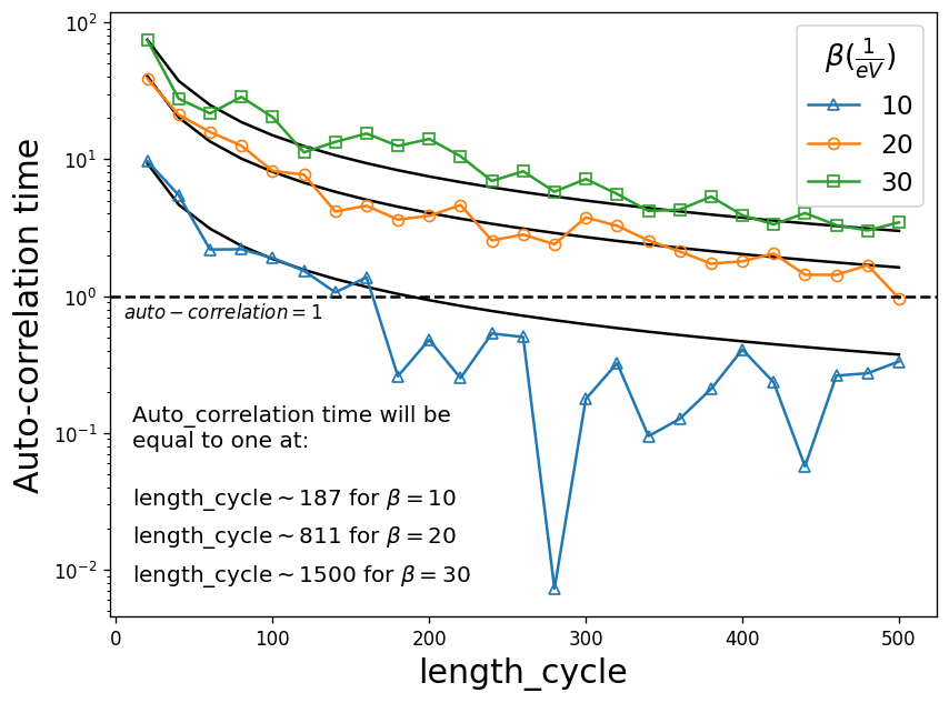
We observe that for example at \(\beta=10\), the converged value of length_cycle (i.e. when auto-correlation time reaches one) is roughly 187. The calculation here has been performed for a fixed value of n_cycles and n_warmup_cycles , whereas they should ideally be increased with increasing \(\beta\).
2. n_warmup_cycles
The system needs to be thermalized first, i.e. for the first few thousand cycles (n_warmup_cycles), we don’t make measurements. In order to have an estimate of how many cycles are needed for thermalization, we set n_warmup_cycle to be zero in the solver and plot the average_order versus the number of cycles. This way, measurements are made from the beginning and the number of cycles at which the average_order starts to saturate is a good estimate for n_warmup_cycles.
[ ]:
t = 1.0    # Half bandwidth
betas = [10, 50, 100]
n_loops = 1
U = 2.0
mu = 0.0
n_cycles = np.arange(100,8000,100)

for b in range(len(betas)):
    if not os.path.exists('../../../data/warm_up_b%i'%betas[b]):
        os.makedirs('../../../data/warm_up_b%i'%betas[b])

    for j in range(len(n_cycles)):
        S = Solver(beta = betas[b], gf_struct = [('up',1), ('down',1)])
        S.G_iw << SemiCircular(2*t)
        # DMFT loop with self-consistency
        for i in range(n_loops):
            print("\n\nIteration = %i / %i" % (i+1, n_loops))
            # Symmetrize the Green's function and use self-consistency
            g = 0.5 * ( S.G_iw['up'] + S.G_iw['down'] )
            for name, g0 in S.G0_iw:
                g0 << inverse( iOmega_n + U/2.0 - mu - t**2 * g )

                # Solve the impurity problem
            S.solve(h_int = U * n('up',0) * n('down',0),   # Local Hamiltonian
                n_cycles  = n_cycles[j],                   # Number of QMC cycles
                length_cycle = 200,                        # Number of Monte Carlo moves in a cycle
                n_warmup_cycles = 0,                       # Warmup cycles
                )
            # Save iterations in archive
            with HDFArchive('../../../data/warm_up_b%i/half-U-wu%i.h5'%(betas[b], n_cycles[j])) as A:
                A['a%i'%i] = S.auto_corr_time
                A['b%i'%i] = S.average_order
[34]:
fig, ax = plt.subplots(1, 1, figsize=(8, 6))
marker=['-^', '-o', '-s']

for b in range(len(betas)):
    average_order = []
    for j in range(len(n_cycles)):
        R = HDFArchive('../../../data/warm_up_b%i/half-U-wu%i.h5'%(betas[b], n_cycles[j]), 'r')
        average_order.append(R['b0'])
    average_order=list(map(lambda x: x/max(average_order), average_order))
    ax.plot(n_cycles, average_order, marker[b], fillstyle="none", label='%i'%betas[b])
ax.set_xscale("log")
ax.set_ylabel('Average_order/maximum_order', fontsize=16)
ax.set_xlabel('n_cycles', fontsize=18)
ax.set_title('n_warmup=0', fontsize=18)
ax.axhline(y=1, linestyle='--', color='k')
plt.legend(title=r'$\beta(\frac{1}{eV})$', title_fontsize=16, fontsize=14)
plt.show()
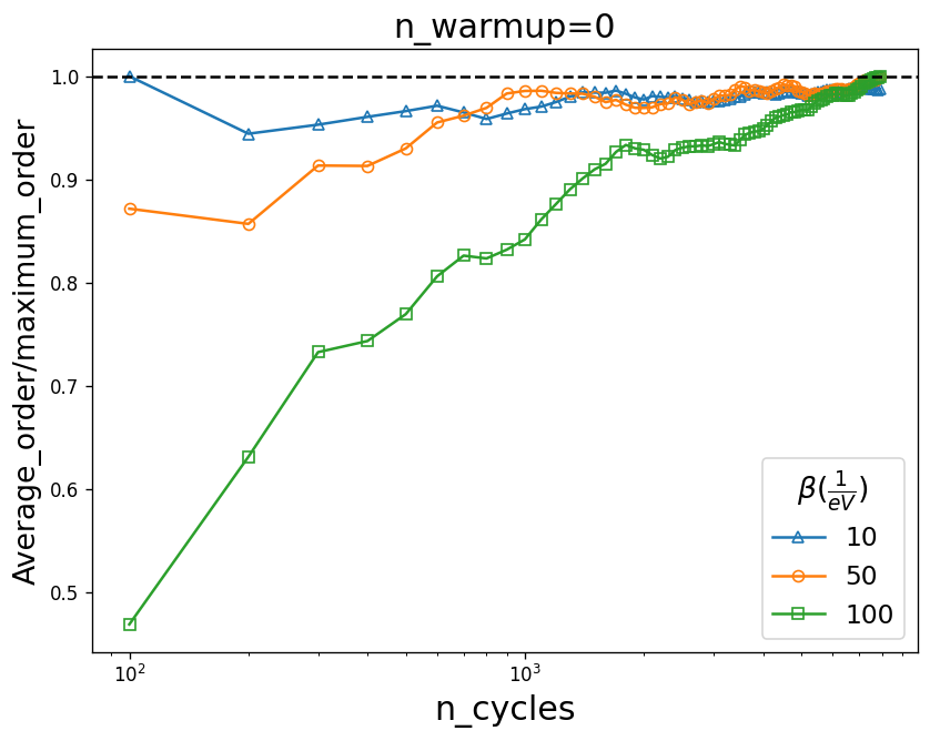
The graph shows that for example at \(\beta=50\) almost 1000 n_warmup_cycles are enough to thermalize the system, but for \(\beta=100\) the thermalization is much slower. Again length_cycles is kept fixed here whereas it varies for different temperatures.
3. n_cycles
The Green’s function in imaginary time \(G(\tau\)) obtained from the solver for different number of n_cycles is plotted. Converged values of length_cycle and n_warmup_cycles are used from the previous tests. The Monte Carlo error should decay as $:nbsphinx-math:sim`$1/sqrt(``n_cycles`).
[ ]:
if not os.path.exists('../../../data/n_cycles_b10'):
    os.makedirs('../../../data/n_cycles_b10')
t = 1.0   # Half bandwidth
beta = 10
n_loops = 1
U = 2.0
n_cycles = [32000, 64000, 128000, 256000, 512000, 1024000, 2048000]

for j in range(len(n_cycles)):
    print('n_cycles =', n_cycles[j])
    S = Solver(beta = beta, gf_struct = [('up',1), ('down',1)])
    S.G_iw << SemiCircular(2*t)

    for i in range(n_loops):

        print("\n\nIteration = %i / %i" % (i+1, n_loops))
        # Symmetrize the Green's function and use self-consistency
        g = 0.5 * ( S.G_iw['up'] + S.G_iw['down'] )
        for name, g0 in S.G0_iw:
            g0 << inverse( iOmega_n + U/2.0 - t**2 * g )

        # Solve the impurity problem
        S.solve(h_int = U * n('up',0) * n('down',0),     # Local Hamiltonian
            n_cycles  = n_cycles[j],                     # Number of QMC cycles
            length_cycle = 187,                          # Number of Monte Carlo moves in a cycle
            n_warmup_cycles = 2000,                      # Warmup cycles
            )

        # Save iterations in archive
        with HDFArchive('../../../data/n_cycles_b10/half-U-nc%ik.h5'%(n_cycles[j]/1000)) as A:
            A['Gtau-%i'%i] = S.G_tau
[38]:
fig, ax = plt.subplots(7, 1, figsize=(6, 11), sharex=True)

for j in range(len(n_cycles)):
    R = HDFArchive('../../../data/n_cycles_b10/half-U-nc%ik.h5'%(n_cycles[j]/1000), 'r')
    ax[j].oplot(R['Gtau-0']['up'].real, '-', label=r"n_cycles = %i"%n_cycles[j])
    ax[j].set_ylabel('')
    ax[j].set_xlabel('')

fig.supylabel(r'$G(\tau)$', x=-0.01, fontsize="18")
fig.supxlabel(r'$\tau$', y= 0.07, fontsize="18")
fig.suptitle(r'$\beta=10 (\frac{1}{eV})$', y=0.93, fontsize="18")
plt.show()
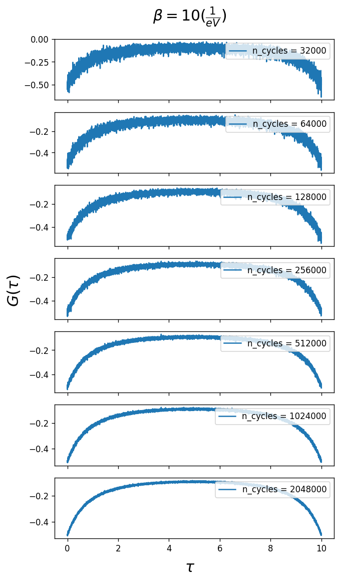
As you can see larger n_cycles gives a smoother Green’s function, i.e. a smaller error on \(G(\tau\)). It depends on the user’s needs in terms of accuracy as to how large n_cycles should be.
4. n_iw
The number of Matsubara frequencies used for the Green’s functions. The Green’s function should decay to zero for large \(i\omega_n\), and capturing this behavior correctly is important for Fourier Transforms and physicality. Here, we plot the electron filling n for different sizes of the frequency mesh. The size of the Matsubara frequency mesh is important when calculating the electron filling n:
The definition of electron filling is \(n = \langle c^\dagger c\rangle\)
and \(\lim_{\tau\to 0} G(\tau) = n\)
\(G(\tau) = -\langle T c(\tau)c^\dagger\rangle = \langle T c^\dagger c(\tau)\rangle \rightarrow G(\tau=0^-) = \langle c^\dagger c\rangle = n\)
The Fourier transform of \(G(\tau=0^-)\) is the sum of \(G(i\omega_n)\) over Matsubara frequencies which is equal to the electron filling.
\(G(\tau=0^-)=\sum_{i\omega_n}{e^{i\omega_n0^-}G(i\omega_n)}=\sum_{i\omega_n}{G(i\omega_n)}\)
$:nbsphinx-math:Rightarrow `$ :math:`n=sum_{iomega_n}{G(iomega_n)}
Therefore density converges only if enough number of Matsubabra frequencies n_iw are kept in the mesh.
[6]:
fig, ax = plt.subplots(1, 2, figsize=(12, 4))
D = 1.5  # Half bandwidth
beta = [100, 1000]
n_max = [20, 40, 80, 160, 320, 640] # Size of the Matsubara frequency mesh
marker=['-^', '-o']
for i in range(len(beta)):
    density = []
    for j in range(len(n_max)):
        iw_mesh = MeshImFreq(beta=beta[i], S='Fermion', n_max=n_max[j])
        G = Gf(mesh=iw_mesh, target_shape=[])
        G << SemiCircular(D)
        density.append(G.density())
    ax[0].set_xscale("log")
    ax[0].plot(n_max, density, marker[i], fillstyle="none", label=beta[i])
    density = list(map(lambda x: x - 0.5, density))
    density = list(map(abs, density))
    ax[1].set_xscale("log")
    ax[1].set_yscale("log")
    ax[1].plot(n_max, density, marker[i], fillstyle="none", label=beta[i])

ax[0].legend(title=r'$\beta(\frac{1}{eV})$', title_fontsize=16, fontsize=14)
ax[0].set_xlabel('$n_{i\omega}$', fontsize=16)
ax[0].set_ylabel('n', fontsize=16)
ax[1].set_ylabel('$|n-0.5|$', fontsize=16)
ax[1].legend(title=r'$\beta(\frac{1}{eV})$', title_fontsize=14, fontsize=12)
ax[1].set_xlabel(r'$n_{i\omega}$', fontsize=16)
plt.show()
WARNING: High frequency moments have an error greater than 1e-4.
 Error = 0.000665894
 Please make sure you treat the constant offset analytically!
WARNING: High frequency moments have an error greater than 1e-4.
 Error = 0.00528623
 Please make sure you treat the constant offset analytically!
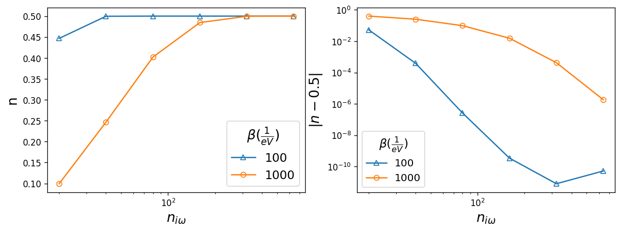
The warning message printed is a hint that the frequency mesh is too small. Since we are working with the semi-circular density of states at half-filling, the electorn filling converges to 0.5. The error on n is plotted on the right which shows that electron filling converges with 320 Matsubara frquencies in the mesh.
So far, we have study the number of Matsubara frequencies only for non-interacting cases. However, interaction can renormalize the shape of the Green’s function, in which case it’s better to directly investigate the Green’s function instead of the electron filling. One can consider that there are enough numbers of Matsubara frequencies in the mesh if the Green’s function is in the \(\frac{1}{\omega}\) decay region (i.e. if the tail of the Green’s function is close to zero).
Below is an example of demonstrating the convergence by looking at the Green’s function (still for the non-interacting case).
[17]:
fig, ax = plt.subplots(figsize=(6, 5))
D = 1.5  # Half bandwidth
beta = 100
n_max = [640, 320, 160, 80, 40, 20]
for j in range(len(n_max)):
    a = np.arange(-n_max[j],n_max[j])
    iw_mesh = MeshImFreq(beta=beta, S='Fermion', n_max=n_max[j])
    G = Gf(mesh=iw_mesh, target_shape=[1,1])
    G << SemiCircular(D)
    ax.plot(a/n_max[j], G.imag.data[:,0], label=n_max[j])

ax.set_xlim(0,)
ax.set_ylim(-1.5,0)
ax.legend(title=r'$n_{i\omega}$', title_fontsize=14, fontsize=12)
ax.set_ylabel("$G(i\omega_n)$", fontsize=16)
ax.set_xlabel("$\omega_n/\omega_{max}$", fontsize=16)
ax.set_title(r'$\beta = %i (\frac{1}{eV})$'%beta, fontsize=16)
plt.show()
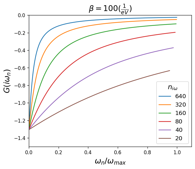
Here the mesh with 640 frequencies is the best choice.
5. n_l
The number of Legendre polynomials to use in accumulations of the Green’s function. Representing the Green’s function in terms of Legendre polynomials is a compact basis representation described in PRB 84, 075145 (2011).
\(G(\mathcal{l})=\sqrt{2l+1}\int_0^{\beta}{d\tau}P_l[x(\tau)]G(\tau)\)
where \(x(\tau)=2\tau/\beta -1\) and \(G(l)\) denotes the coefficients of \(G(\tau)\) in Legendre basis.
We first need to define a function that transforms the Green’s function from the imaginary time domain to the Legendre basis.
[2]:
from triqs.gfs.tools import fit_legendre

def ImTime_to_Legendre(G_tau, order=100, G_l_cut=1e-19):
    """ Filter binned imaginary time Green's function
    using a Legendre filter of given order and coefficient threshold.
    """

    g_l = fit_legendre(G_tau, order=order)
    g_l['up'].data[:] *= (np.abs(g_l['up'].data) > G_l_cut)
    g_l['up'].enforce_discontinuity(np.identity(G_tau['up'].target_shape[0]))

    return g_l
Next, the Green’s function in imaginary time \(G(\tau\)) is obtained from the solver at \(\mathcal{\beta} = 50 (1/eV)\) and n_l=60. We use the function defined in the previous cell to transform \(G(\tau)\) to the Legendre basis.
[ ]:
import os
if not os.path.exists('../../../data/g_l'):
    os.makedirs('../../../data/g_l')

# Parameters of the model
t = 1.0
beta = 50
n_loops = 1
U = 2.0
n_l = 60
# Construct the impurity solver
S = Solver(beta = beta, n_l=n_l, gf_struct = [('up',1), ('down',1)])
# This is a first guess for G
S.G_iw << SemiCircular(2*t)

for i in range(n_loops):

    g = 0.5 * ( S.G_iw['up'] + S.G_iw['down'] )
    for name, g0 in S.G0_iw:
        g0 << inverse( iOmega_n + U/2.0 - t**2 * g )

    # Solve the impurity problem
    S.solve(h_int = U * n('up',0) * n('down',0),   # Local Hamiltonian
        n_cycles  = 256000,                           # Number of QMC cycles
        length_cycle = 200,
        n_warmup_cycles = 4000,                      # Warmup cycles
        )

    # Save iteration in archive
    with HDFArchive("../../../data/g_l/half-U-nl%i.h5"%n_l) as A:
        A['Gtau-%i'%i] = S.G_tau
[6]:
R = HDFArchive('../../../data/g_l/half-U-nl%i.h5'%n_l, 'r')
G_l = ImTime_to_Legendre(R['Gtau-0'], order=n_l, G_l_cut=1e-19)
The cell below separates the odd and even parts of the Legendre Green’s function and the plot tells us how many Legendre plynomials we need to keep in our calcualtion. The cut-off point determines the error on \(G(l)\) and the solver more or less. The coefficients for odd l must be zero due to particle-hole symmetry.
[8]:
fig, ax1 = plt.subplots(figsize=(8, 6))
left, bottom, width, height = [0.38, 0.2, 0.5, 0.45]
ax2 = fig.add_axes([left, bottom, width, height])
d_even=[]
d_odd=[]
dim=G_l['up'].data.shape[0]
x_even=np.arange(0,dim,2)
x_odd=np.arange(1,dim,2)
for i in range(0,dim,2):
    d_even.append(G_l['up'].real.data[i,0])
for k in range(1,dim,2):
    d_odd.append(G_l['up'].real.data[k,0])
ax1.plot(x_even, d_even, marker=MarkerStyle('o', fillstyle='bottom'), label='l even')
ax1.plot(x_odd, d_odd, '-^', label='l odd')
d_even_abs= list(map(abs, d_even))
d_odd_abs= list(map(abs, d_odd))
ax2.plot(x_even, d_even_abs, marker=MarkerStyle('o', fillstyle='bottom'))
ax2.plot(x_odd, d_odd_abs, '-^')
pyplot.yscale('log')
ax1.set_ylim(-6,1.5)
ax1.legend(loc=(0.8,0.85))
ax1.set_xlabel('$l$', fontsize=18)
ax1.set_ylabel('$G(l)$', fontsize=18)
ax2.set_ylabel('$|G(l)|$', fontsize=14)
plt.show()
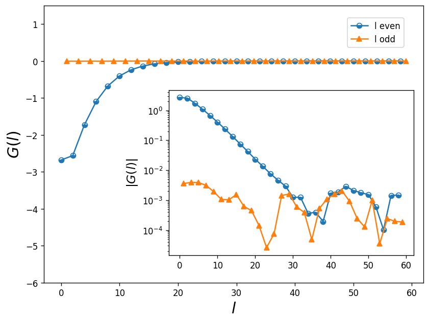
From inspecting this graph, it is clear that 35 coefficients (l) are enough to reach convergence. We can efficiently use this procedure as a noise filter by cutting the number of coefficients after \(G(l)\) reaches its minimum value.
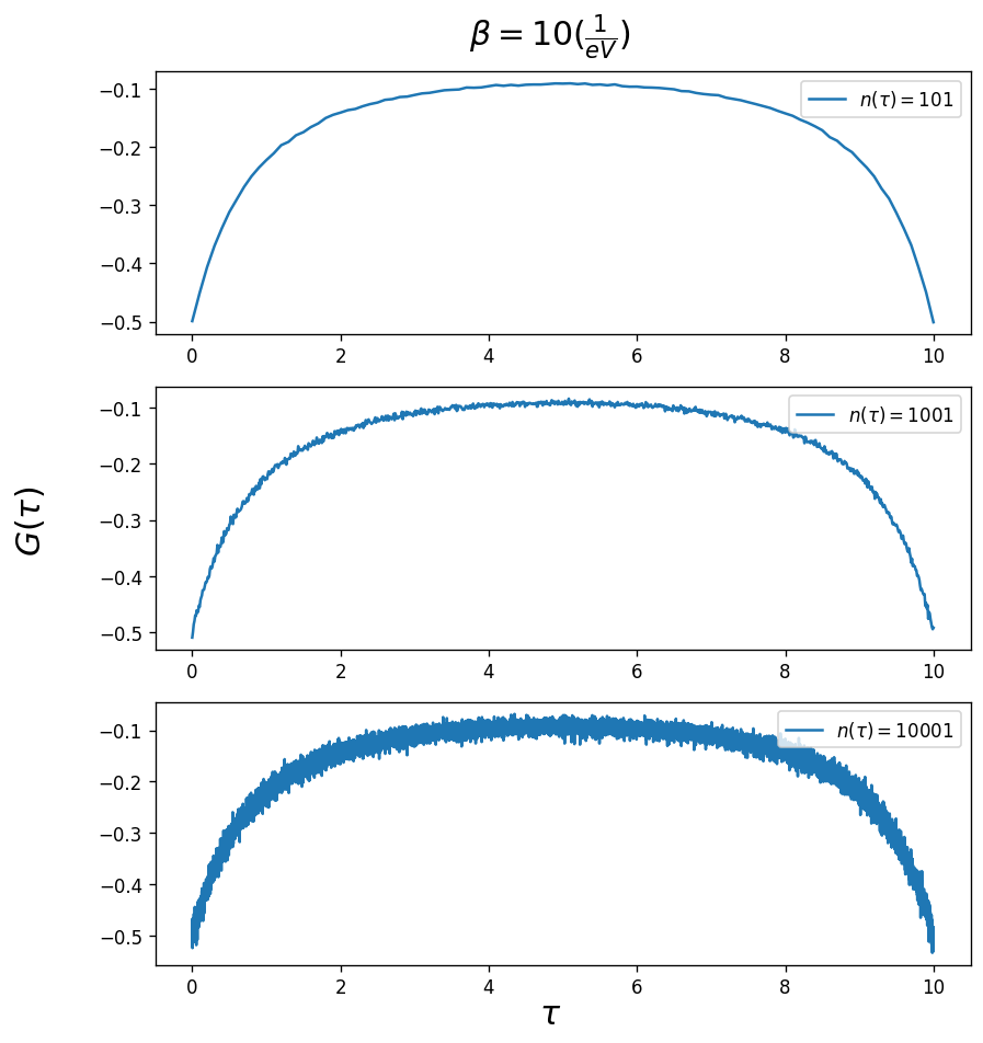
6. n_tau
Number of imaginary time points used for the Green’s function. The CTHYB solver calculates the Green’s function at time differences that are randomly sampled, \(G(\tau_i-\tau_j)\) (where \(\tau_i\) and \(\tau_j\) are randomly chosen between 0 and \(\beta\)). Every \(\tau\) value of the grid is associated with a bin of a given width. If the number of \(\tau\) points that fall into each bin is small (or in other words there are a lot of bins, n_tau is large) then the
error in that bin will be large. Therefore, the plot of \(G(\tau)\) will show a lot of noise as n_tau is increased. However this does not matter because applying a Fourier transform on the Green’s function sums over all the bins and averages out the error. In fact n_tau should be as large as possible.
[ ]:
import os
if not os.path.exists('../../../data/ntau-b10'):
    os.makedirs('../../../data/ntau-b10')

# Parameters of the model
t = 1.0
beta = 10
n_loops = 1
U = 2.0
n_tau = [101, 1001, 10001]
# Construct the impurity solver

for j in range(len(n_tau)):
    # n_iw=math.floor((1/8)*n_tau[j])
    print('n_tau =', n_tau[j])
    S = Solver(beta = beta, n_iw=50, n_tau=n_tau[j], gf_struct = [('up',1), ('down',1)])
    # This is a first guess for G
    S.G_iw << SemiCircular(2*t)

    for i in range(n_loops):

        g = 0.5 * ( S.G_iw['up'] + S.G_iw['down'] )
        for name, g0 in S.G0_iw:
            g0 << inverse( iOmega_n + U/2.0 - t**2 * g )

        # Solve the impurity problem
        S.solve(h_int = U * n('up',0) * n('down',0),   # Local Hamiltonian
            n_cycles  = 256000,                           # Number of QMC cycles
            length_cycle = 200,
            n_warmup_cycles = 4000,                      # Warmup cycles
            )

        # Save iteration in archive
        with HDFArchive("../../../data/ntau-b10/half-U-ntau%i.h5"%n_tau[j]) as A:
            A['Gtau-%i'%i] = S.G_tau
[3]:
fig, ax = plt.subplots(3, 1, figsize=(8, 9))
n_tau = [101, 1001, 10001]
for j in range(len(n_tau)):
    A1 = HDFArchive("../../../data/ntau-b10/half-U-ntau%i.h5"%n_tau[j], 'r')
    ax[j].oplot(A1['Gtau-0']['up'].real, '-', label=r"$n(\tau) = %i$"%n_tau[j])
    ax[j].set_ylabel('')
    ax[j].set_xlabel('')
fig.supylabel(r'$G(\tau)$', x=-0.01, fontsize="18")
fig.supxlabel(r'$\tau$', y= 0.07, fontsize="18")
fig.suptitle(r'$\beta=10 (\frac{1}{eV})$', y=0.93, fontsize="18")
plt.show()
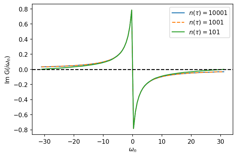
Applying Fourier transform on the Green’s function to go from imaginary time to imaginary frequency domain also shows that it is better to work with larger n_tau. As can be seen from the graph below, for small n_tau the Green’s function crosses zero which is not physical.
[20]:
from triqs.gfs import Fourier
from triqs.gfs import make_gf_from_fourier
[21]:
fig, ax = plt.subplots(1, 1, dpi=150, figsize=(6, 4))
iw_mesh = MeshImFreq(beta=10, S='Fermion', n_max=50)
gf_struct = [('g',1)]
ls=['-', '--', '-']
Giw = BlockGf(mesh=iw_mesh, gf_struct=gf_struct)
n_tau = [10001, 1001, 101]
for j in range(len(n_tau)):
    A1 = HDFArchive("../../../data/ntau-b10/half-U-ntau%i.h5"%n_tau[j], 'r')
    Giw << Fourier(A1['Gtau-0'])
    ax.oplot(Giw.imag, label=r"$n(\tau) = %i$"%n_tau[j], linestyle=ls[j])
ax.axhline(y=0, linestyle='--', color='k')
plt.show()
WARNING: Direct Fourier cannot deduce the high-frequency moments of G(tau) due to noise or a coarse tau-grid.     Please specify the high-frequency moments for higher accuracy.
WARNING: Direct Fourier cannot deduce the high-frequency moments of G(tau) due to noise or a coarse tau-grid.     Please specify the high-frequency moments for higher accuracy.
WARNING: Direct Fourier cannot deduce the high-frequency moments of G(tau) due to noise or a coarse tau-grid.     Please specify the high-frequency moments for higher accuracy.
[Direct Fourier] WARNING: The imaginary time mesh is less than six times as long as the number of positive frequencies.
This can lead to substantial numerical inaccuracies at the boundary of the frequency mesh.