The Anderson impurity model
To illustrate how the CTQMC solver works in practice, we show the example of a one-orbital Anderson impurity embedded in a flat (Wilson) conduction bath. The interacting part of the local Hamiltonian of this problem is simply:
and the non-interacting Green’s function is:
In this example, there is a Coulomb interaction \(U\) on the impurity level,
which is at an energy \(\epsilon_f\). The bath Green’s function is \(\Gamma(i
\omega_n)\), and it has a flat density of states over the interval
\([-1,1]\). Finally, \(V\) is the hybridization amplitude between the
impurity and the bath. Let us solve this problem with the CTQMC solver. Here is
the python script:
from triqs.gfs import *
from triqs.operators import *
from triqs_cthyb import Solver
from h5 import HDFArchive
import triqs.utility.mpi as mpi

# Parameters
D, V, U = 1.0, 0.2, 4.0
e_f, beta = -U/2.0, 50

# Construct the impurity solver with the inverse temperature
# and the structure of the Green's functions
S = Solver(beta = beta, gf_struct = [ ('up',1), ('down',1) ], n_l = 100)

# Initialize the non-interacting Green's function S.G0_iw
for name, g0 in S.G0_iw: g0 << inverse(iOmega_n - e_f - V**2 * Wilson(D))

# Run the solver. The results will be in S.G_tau, S.G_iw and S.G_l
S.solve(h_int = U * n('up',0) * n('down',0),     # Local Hamiltonian
        n_cycles  = 500000,                      # Number of QMC cycles
        length_cycle = 200,                      # Length of one cycle
        n_warmup_cycles = 10000,                 # Warmup cycles
        measure_G_l = True)                      # Measure G_l

# Save the results in an HDF5 file (only on the master node)
if mpi.is_master_node():
    with HDFArchive("aim_solution.h5",'w') as Results:
        Results["G_tau"] = S.G_tau
        Results["G_iw"] = S.G_iw
        Results["G_l"] = S.G_l
Running this script on a single processor takes about 5 minutes and generates
an HDF5 archive file called aim_solution.h5. This file contains the Green’s
function in imaginary time, in imaginary frequencies, and in Legendre polynomial basis
found by the solver.
Let us plot the Green’s function:
from triqs.gfs import *
from h5 import *
from triqs.plot.mpl_interface import oplot

with HDFArchive('aim_solution.h5','r') as ar:
    oplot(ar['G_iw']['up'], '-o', x_window = (0,10))
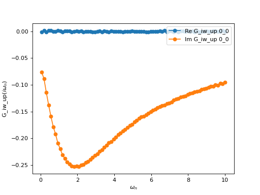
As expected the result shows a particle-hole symmetric impurity Green’s function (the real part vanishes up to the statistical noise).
Let us now go through the script in some more details.
from triqs.gfs import *
from triqs.operators import *
from triqs_cthyb import Solver
from h5 import HDFArchive
import triqs.utility.mpi as mpi
These lines import the classes to manipulate Green’s functions, fermionic operators, and the CTQMC solver.
# Parameters
D, V, U = 1.0, 0.2, 4.0
e_f, beta = -U/2.0, 50
This just sets the parameters of the problem.
# Construct the impurity solver with the inverse temperature
# and the structure of the Green's functions
S = Solver(beta = beta, gf_struct = [ ('up',1), ('down',1) ], n_l = 100)
This is the construction of the Solver object. The class is described
in more detail in Solver. Basically, the constructor
of the Solver needs two keywords:
beta: the inverse temperature,gf_struct: a list of pairs [ (str, int), …] describing the block structure of the Green’s function.
This ensures that all quantities within Solver are correctly initialised, and in particular that the block structure of all Green’s function objects is consistent.
After the Solver is constructed it needs to know what the non-interacting Green’s function
of the impurity is. From this information, the Solver will deduce the hybridization function
which is used in the algorithm. The non-interacting Green’s function must be put in the
class member S.G0_iw:
# Initialize the non-interacting Green's function S.G0_iw
for name, g0 in S.G0_iw: g0 << inverse(iOmega_n - e_f - V**2 * Wilson(D))
At this stage, everything is ready for the Solver and we just run it calling its member
function solve:
# Run the solver. The results will be in S.G_tau, S.G_iw and S.G_l
S.solve(h_int = U * n('up',0) * n('down',0),     # Local Hamiltonian
        n_cycles  = 500000,                      # Number of QMC cycles
        length_cycle = 200,                      # Length of one cycle
        n_warmup_cycles = 10000,                 # Warmup cycles
        measure_G_l = True)                      # Measure G_l
The run is controlled by the parameters of solve():
h_int: The interacting part of the local Hamiltonian written with TRIQS operators.n_cycles: The number of Monte Carlo cycles.length_cycle: The number of Monte Carlo moves in a cycle.random_name: The name of the random number generator.measure_g_l: We want to accumulate the Green’s function in a basis of Legendre polynomials.
When solve() has finished, it puts the result for the interacting Green’s
function in imaginary time in its member S.G_tau and the Green’s function
in imaginary frequencies in S.G_iw. The last lines of the script save the
Green’s function in the HDF archive.