Setting the parameters
Here’s a step-by-step guide that should show you how to prepare a CTQMC run. Take the time to go through this little guide as it can help you avoid doing simple mistakes.
Step 1 - construct the solver instance
At first you need to create an instance of the CTQMC solver class. This is done with:
from triqs.operators import *
from triqs_cthyb import Solver

# Create a solver instance
S = Solver(beta = beta, gf_struct = gf_struct)
The first parameter of the solver is the inverse temperature. In order to
complete the construction of the instance, you need to figure out what is the
correct structure of the Green’s function for the problem you are considering.
You should always try to take advantage of a possible block structure of the
Green’s function. In a spin-conserving system, the Green’s function can often
be (at least) cut into up and down spin sectors. When the structure is
clear you can set the parameter gf_struct, which is a list() or pairs,
each containing the name of the block and the size of the block.
Examples
For a single-band Hubbard model with a local Coulomb interaction, the Green’s function can be cut in two up/down blocks of size 1. We would have:
gf_struct = [ ('up', 1), ('down', 1) ]
For a two-band Hubbard model with a hybridization between the bands, the Green’s function can be cut in two up/down blocks, but there are off-diagonal orbital elements. We have:
gf_struct = [ ('up', 2), ('down', 2) ]
Step 2 - the Hamiltonian
The solver instance is ready. Now you need to prepare all the parameters
that will enter the solve() method and start the calculation. So
the next step is to describe the local Hamiltonian. This is the Hamiltonian
acting on the effective impurity sites/orbitals. It is very important to
include only the quartic terms and not the quadratic terms in this
Hamiltonian. The latter terms will be computed from the kownledge of the
non-interacting Green’s function S.G0_iw as explained below (see Step 7). The
interacting Hamiltonian is given in the parameter h_int.
with the use of second-quantization operators.
The arguments in the parenthesis of the c(), c_dag()
and n() operators must be compatible with the structure of the Green’s
function gf_struct.
Examples
For a single-band Hubbard model with a local Coulomb interaction:
h_int = U * n('up',0) * n('down',0)
Two-orbital Hubbard model, no inter-orbital interaction, but a hybridization between the bands (this term will not appear in the local Hamiltonian!):
h_int = U * (n('up',0) * n('down',0) + n('up',1) * n('down',1))
Step 3 - the Monte Carlo parameters
There are three parameters that control how many steps and measures are done
during the Monte Carlo sampling. n_cycles is the total number of measurement
cycles done. A cycle has length_cycle Monte Carlo moves in it. The
measurements start after n_warmup_cycles cycles have been made and there is
a measurement at the end of every cycle. At the end of the run, there will be
n_cycles measurements and a total of (n_warmup_cycles + n_cycles) x
length_cycle) moves.
When the solver is spread on a parallel machine, each core will do n_cycles
measurements cycles and n_warmup_cycles warmup cycles. Therefore the same
input run on a larger number of cores will yield a larger statistics.
Step 6 - Legendre or not?
The CTQMC algorithm computes the Green’s function on the imaginary-time
interval \([0,\beta]\). By default, \(G(\tau)\) is computed by binning
measurements in \(n_{\tau}\) bins. However, in order to gain memory and to
reduce high-frequency noise, the Green’s function may be expanded on a basis of
n_l Legendre polynomials by setting the parameter measure_g_l to True.
The question is, how many of these polynomials should one use? Our
recommendation is to do a first test run with a large number of coefficients,
say 80. When the run is over, one can inspect the Legendre Green’s function and
decide how many coefficients should be kept. This will be detailed below.
Step 7 - prepare the non-interacting Green’s function
The last step before starting the solver is to prepare the non-interacting
Green’s function of the problem. From the knowledge of this Green’s function,
the solver can extract the hybridization function used in the algorithm and the
quadratic terms of the local Hamiltonian. The non-interacting Green’s function
must be initialized in the member G0_iw of the solver instance. For example,
one would write
for name, g0 in S.G0_iw:
  g0 << inverse(iOmega_n - e_f - V**2 * Wilson(D))
to initialize the Green’s function of an impurity embedded in a flat conduction bath.
Step 8 - we’re ready to go!
Everything is ready at this stage and you just need to call the solve()
member of the solver with all the information you prepared, e.g.:
S.solve(h_int = U * n('up',0) * n('down',0),
        n_cycles  = 500000,
        length_cycle = 200,
        n_warmup_cycles = 10000)
or alternatively by predefining a dict of params:
p = {}
p['n_warmup_cycles'] = 10000
p['n_cycles'] = 500000
p['length_cycle'] = 200
S.solve(h_int = U * n('up',0) * n('down',0), **p)
When you call the solver, the local Hamiltonian (with the quadratic terms) is shown. Be careful to check that this is indeed the Hamiltonian that you expect! At the end of the run, the solver has computed the following objects:
The interacting Green’s function of the problem on the imaginary time axis. This is in the class member
G_tau.The interacting Green’s function of the problem on the Matsubara frequency axis. This is in the class member
G_iw.The interacting Legendre Green’s function of the problem, if measure_g_l=True. This is put in the member
G_l. This output is useful to decide how many Legendre coefficients should be used.
Final Step - analyze the output
One of the most important checks that needs to be done is to ensure that the
high-frequency behaviour of your imaginary frequency Green’s function and
self-energy are correct and lead to physically sensible values. You should use
the fitting function tail_fit (provided in triqs.gfs) to determine the
optimal fitting parameters fit_min_n and fit_max_n.
This post-processing task can also be delegated to the Solver object by
setting perform_tail_fit = True and other solve()
parameters related to tail fitting.
If you use the Legendre expansion, you should also decide on the ideal number of Legendre coefficients to keep for the following runs. If you have saved the Legendre Green’s function in an archive, you can then plot it:
from triqs.gfs import *
from h5 import *
from triqs.plot.mpl_interface import oplot

A = HDFArchive("aim_solution.h5",'r')
oplot(A['G_l']['up'], '-o', x_window=(15,45) )
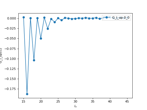
From this plot you see that for \(l > 30\), the value of the
coefficient is of the order of the statistical noise. There is therefore no
information in the coefficients with \(l > 30\) and one can set
n_l = 30 for the following runs. Of course, if you are going to use
more statistics or a larger number of cores, you may have to readjust this
value.