Building DMFT calculations

TRIQS includes all basic ingredients to write DMFT computations: Green’s functions and impurity solvers. The self-consistency condition is assembled from these ingredients, using the basic operations on Green’s function (arithmetic operations, slicing, …).

There is no general DMFT computation class that would handle all cases, just the bricks to build them easily. Here’s an example:

Plain-vanilla DMFT: the Bethe lattice

Here is a complete computation of a single-site DMFT on a Bethe lattice [script]:

from triqs.gf import *
from triqs.operators import *
from h5 import *
import triqs.utility.mpi as mpi
from triqs_cthyb import Solver

# Set up a few parameters
U = 2.5
half_bandwidth = 1.0
chemical_potential = U/2.0
beta = 100
n_loops = 5

# Construct the CTQMC solver
S = Solver(beta = beta, gf_struct = [ ('up',1), ('down',1) ])

# Initalize the Green's function to a semi circular DOS
S.G_iw << SemiCircular(half_bandwidth)

# Now do the DMFT loop
for i_loop in range(n_loops):

    # Compute new S.G0_iw with the self-consistency condition while imposing paramagnetism
    g = 0.5 * (S.G_iw['up'] + S.G_iw['down'])
    for name, g0 in S.G0_iw:
        g0 << inverse(iOmega_n + chemical_potential - (half_bandwidth/2.0)**2 * g)

    # Run the solver
    S.solve(h_int = U * n('up',0) * n('down',0),    # Local Hamiltonian
            n_cycles = 5000,                        # Number of QMC cycles
            length_cycle = 200,                     # Length of a cycle
            n_warmup_cycles = 1000)                 # How many warmup cycles

    # Some intermediate saves
    if mpi.is_master_node():
        with HDFArchive("dmft_solution.h5") as ar:
            ar["G_tau-%s"%i_loop] = S.G_tau
            ar["G_iw-%s"%i_loop] = S.G_iw
            ar["Sigma_iw-%s"%i_loop] = S.Sigma_iw

    # Here we could write some convergence test
    # if converged : break

The solver has been discussed above, so let us just emphasize that the DMFT loop itself is polymorphic: it would run as well with any other solver, as long as it provides G0_iw and G_tau attributes. Even if here the self-consistency condition is very simple, this property would still be true in more complex cases.

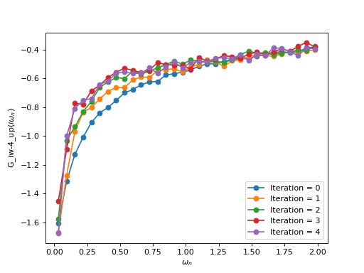
This run generates a file single_site_bethe.h5 containing the Green’s function at every iteration. You can plot them to see the convergence on the solver:

from triqs.gf import *
from h5 import *
from triqs.plot.mpl_interface import oplot, plt

with HDFArchive("dmft_solution.h5",'r') as ar:
    for i in range(5):
        oplot(ar['G_iw-%i'%i]['up'], '-o', mode = 'I',
              label = 'Iteration = %s'%i,
              x_window = (0,2))

plt.legend(loc=4)