Multiorbital impurity model
We present another more complex example here. This time, we solve the five-band impurity with a fully-rotationally invariant interaction:
\[\mathcal{H}_\mathrm{int} = \frac{1}{2} \sum_{ijkl,\sigma \sigma'} U_{ijkl} a_{i \sigma}^\dagger a_{j \sigma'}^\dagger a_{l \sigma'} a_{k \sigma}.\]
Here is the python script:
from triqs.gfs import *
from h5 import HDFArchive
from triqs_cthyb import Solver
import triqs.operators.util as op
import triqs.utility.mpi as mpi

# General parameters
filename = 'slater_five_band.h5'             # Name of file to save data to
beta = 40.0                                  # Inverse temperature
l = 2                                        # Angular momentum
n_orb = 2*l + 1                              # Number of orbitals
U = 4.0                                      # Screened Coulomb interaction
J = 1.0                                      # Hund's coupling
half_bandwidth = 1.0                         # Half bandwidth
mu = 25.0                                    # Chemical potential
spin_names = ['up','down']                   # Outer (non-hybridizing) blocks
off_diag = False                             # Include orbital off-diagonal elements?
n_loop = 2                                   # Number of DMFT self-consistency loops

# Solver parameters
p = {}
p["n_warmup_cycles"] = 10000     # Number of warmup cycles to equilibrate
p["n_cycles"] = 100000           # Number of measurements
p["length_cycle"] = 500          # Number of MC steps between consecutive measures
p["move_double"] = True          # Use four-operator moves

# Block structure of Green's functions
# gf_struct = [ ('up',5), ('down',5) ]
# This can be computed using the TRIQS function as follows:
gf_struct = op.set_operator_structure(spin_names,n_orb,off_diag=off_diag)

# Construct the 4-index U matrix U_{ijkl}
# The spherically-symmetric U matrix is parametrised by the radial integrals
# F_0, F_2, F_4, which are related to U and J. We use the functions provided
# in the TRIQS library to construct this easily:
U_mat = op.U_matrix(l=l, U_int=U, J_hund=J, basis='spherical')

# Set the interacting part of the local Hamiltonian
# Here we use the full rotationally-invariant interaction parametrised
# by the 4-index tensor U_{ijkl}.
# The TRIQS library provides a function to build this Hamiltonian from the U tensor:
H = op.h_int_slater(spin_names,n_orb,U_mat,off_diag=off_diag)

# Construct the solver
S = Solver(beta=beta, gf_struct=gf_struct)

# Set the hybridization function and G0_iw for the Bethe lattice
delta_iw = GfImFreq(indices=[0], beta=beta)
delta_iw << (half_bandwidth/2.0)**2 * SemiCircular(half_bandwidth)
for name, g0 in S.G0_iw: g0 << inverse(iOmega_n + mu - delta_iw)

# Now start the DMFT loops
for i_loop in range(n_loop):

  # Determine the new Weiss field G0_iw self-consistently
  if i_loop > 0:
    g_iw = GfImFreq(indices=[0], beta=beta)
    # Impose paramagnetism
    for name, g in S.G_tau: g_iw << g_iw + (0.5/n_orb)*Fourier(g)
    # Compute S.G0_iw with the self-consistency condition
    for name, g0 in S.G0_iw:
        g0 << inverse(iOmega_n + mu - (half_bandwidth/2.0)**2 * g_iw )

  # Solve the impurity problem for the given interacting Hamiltonian and set of parameters
  S.solve(h_int=H, **p)

  # Save quantities of interest on the master node to an h5 archive
  if mpi.is_master_node():
      with HDFArchive(filename,'a') as Results:
          Results['G0_iw-%s'%i_loop] = S.G0_iw
          Results['G_tau-%s'%i_loop] = S.G_tau
This script generates an HDF5 archive file called slater_five_band.h5.
This file contains the Green’s function in imaginary time and in imaginary
frequencies found by the solver. Let us plot the Green’s function:
from triqs.gfs import *
from triqs.gfs.gf_fnt import rebinning_tau
from h5 import *
from triqs.plot.mpl_interface import oplot

with HDFArchive('slater_five_band.h5','r') as ar:
    # Calculate orbital- and spin-averaged Green's function
    G_tau = ar['G_tau-1']
    g = G_tau['up_0']
    # This gives a complex valued gf (required by rebinning_tau)
    g_tau_ave = Gf(mesh=g.mesh, target_shape=g.target_shape)
    for name, g in G_tau: g_tau_ave += g
    g_tau_ave = g_tau_ave/10.
    g_tau_rebin = rebinning_tau(g_tau_ave,1000)
    g_tau_rebin.name = r'$G_{\rm ave}$'
    oplot(g_tau_rebin,linewidth=2,label='G_avg')
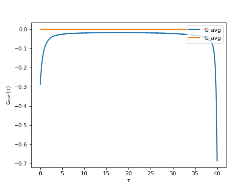
We have rebinned the data to 1000 points to reduce the noise. The calculation takes about an hour and data was accumulated on 32 cores.