5. Plotting the spectral function

In this tutorial we go through the steps to plot tight-binding bands from a Wannier90 Hamiltonian and spectralfunctions with analytically continued (real-frequency) self-energies obtained from DMFT.

%matplotlib inline
from IPython.display import display
from IPython.display import Image
import numpy as np
import importlib, sys
import matplotlib.pyplot as plt
from matplotlib import cm
from timeit import default_timer as timer

from ase.io.espresso import read_espresso_in

from h5 import HDFArchive
from solid_dmft.postprocessing import plot_correlated_bands as pcb

1. Configuration

The script makes use of the triqs.lattice.utils class, which allows to set up a tight-binding model based on a Wannier90 Hamiltonian. Additionally, you may upload a self-energy in the usual solid_dmft format to compute correlated spectral properties. Currently, the following options are implemented:

1. bandstructure

2. Fermi slice

Basic options

We start with configuring these options. For this example we try a tight-binding bandstructure including the correlated bands (kslice = False, 'tb': True, 'alatt': True), but feel free to come back here to explore. Alternatively to an intensity plot of the correlated bands (qp_bands), you can compute the correlated quasiparticle bands assuming a Fermi liquid regime.

The options for \(\Sigma(\omega)\) are calc or model, which performs a Fermi liquid linearization in the low-frequency regime. The latter will be reworked, so better stick with calc for now.

kslice = False

bands_config = {'tb': True, 'alatt': True, 'qp_bands': False, 'sigma': 'calc'}
kslice_config = {'tb': True, 'alatt': True, 'qp_bands': False, 'sigma': 'calc'}
config = kslice_config if kslice else bands_config

Wannier90

Next we will set up the Wannier90 Input. Provide the path, seedname, chemical potential and orbital order used in Wannier90. You may add a spin-component, and any other local Hamiltonian. For t2g models the orbital order can be changed (to orbital_order_to) and a local spin-orbit coupling term can be added (add_lambda). The spectral properties can be viewed projected on a specific orbital.

w90_path = './'
w90_dict = {'w90_seed': 'svo', 'w90_path': w90_path, 'mu_tb': 12.3958, 'n_orb': 3,
            'orbital_order_w90': ['dxz', 'dyz', 'dxy'], 'add_spin': False}

orbital_order_to = ['dxy', 'dxz', 'dyz']
proj_on_orb = None # or 'dxy' etc

BZ configuration

Optional: ASE Brillouin Zone

It might be helpful to have a brief look at the Brillouin Zone by loading an input file of your favorite DFT code (Quantum Espresso in this case). ASE will write out the special \(k\)-points, which we can use to configure the BZ path. Alternatively, you can of course define the dictionary kpts_dict yourself. Careful, it might not define \(Z\), which is needed and added below.

scf_in = './svo.scf.in'

# read scf file
atoms = read_espresso_in(scf_in)
# set up cell and path
lat = atoms.cell.get_bravais_lattice()
path = atoms.cell.bandpath('', npoints=100)
kpts_dict = path.todict()['special_points']

for key, value in kpts_dict.items():
    print(key, value)
lat.plot_bz()

G [0. 0. 0.]
M [0.5 0.5 0. ]
R [0.5 0.5 0.5]
X [0.  0.5 0. ]

<Axes3DSubplot:>

---

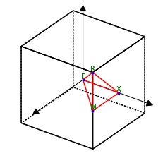
Depending on whether you select kslice=True or False, a corresponding tb_config needs to be provided containing information about the \(k\)-points, resolution (n_k) or kz-plane in the case of the Fermi slice. Here we just import the \(k\)-point dictionary provided by ASE above and add the \(Z\)-point. If you are unhappy with the resolution of the final plot, come back here and crank up n_k. For the kslice, the first letter corresponds to the upper left corner of the plotted Brillouin zone, followed by the lower left corner and the lower right one (\(Y\), \(\Gamma\), and \(X\) in this case).

# band specs
tb_bands = {'bands_path': [('R', 'G'), ('G', 'X'), ('X', 'M'), ('M', 'G')], 'Z': np.array([0,0,0.5]), 'n_k': 50}
tb_bands.update(kpts_dict)

# kslice specs
tb_kslice = {key: tb_bands[key] for key in list(tb_bands.keys()) if key.isupper()}
kslice_update = {'bands_path': [('Y', 'G'),('G', 'X')], 'Y': np.array([0.5,0.0,0]), 'n_k': 50, 'kz': 0.0}
tb_kslice.update(kslice_update)

tb_config = tb_kslice if kslice else tb_bands

Self-energy

Here we provide the info needed from the h5Archive, like the self-energy, iteration count, spin and block component and the frequency mesh used for the interpolation. The values for the mesh of course depend on the quantity of interest. For a kslice the resolution around \(\omega=0\) is crucial and we need only a small energy window, while for a bandstructure we are also interested in high energy features.

freq_mesh_kslice = {'window': [-0.5, 0.5], 'n_w': int(1e6)}
freq_mesh_bands = {'window': [-5, 5], 'n_w': int(1e3)}
freq_mesh = freq_mesh_kslice if kslice else freq_mesh_bands

dmft_path = './svo_example.h5'

proj_on_orb = orbital_order_to.index(proj_on_orb) if proj_on_orb else None
sigma_dict = {'dmft_path': dmft_path, 'it': 'last_iter', 'orbital_order_dmft': orbital_order_to, 'spin': 'up',
              'block': 0, 'eta': 0.0, 'w_mesh': freq_mesh, 'linearize': False, 'proj_on_orb' : proj_on_orb}

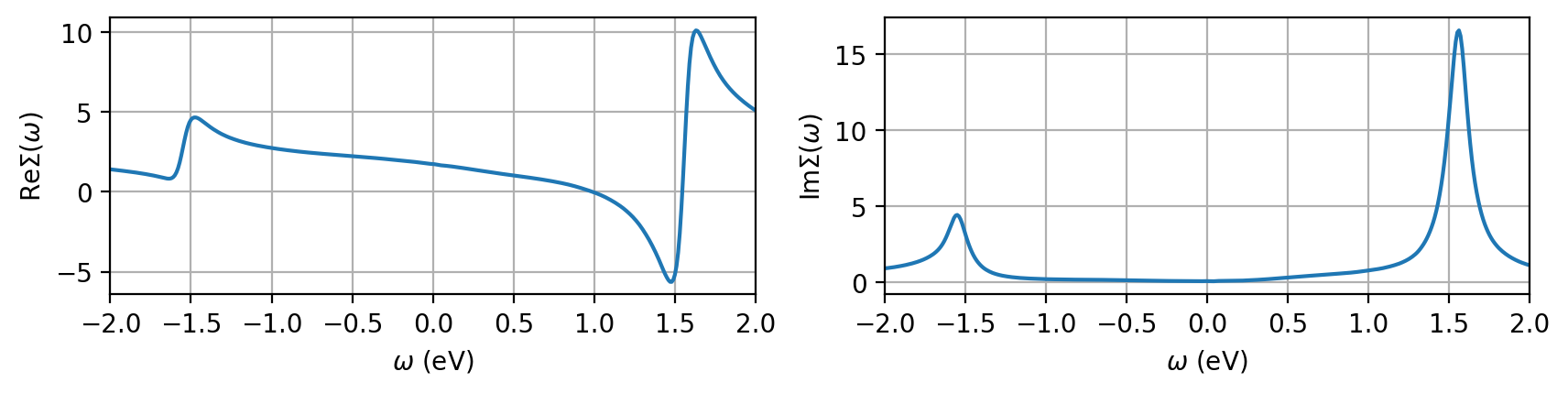
Optional: for completeness and as a sanity check we quickly take a look at the self-energy. Make sure you provide a physical one!

with HDFArchive(dmft_path, 'r') as h5:
    sigma_freq = h5['DMFT_results']['last_iter']['Sigma_freq_0']

fig, ax = plt.subplots(1, 2, figsize=(10,2), squeeze=False, dpi=200)

orb = 0
sp = 'up_0'
freq_mesh = np.array([w.value for w in sigma_freq[sp][orb,orb].mesh])

ax[0,0].plot(freq_mesh, sigma_freq[sp][orb,orb].data.real)
ax[0,1].plot(freq_mesh, -sigma_freq[sp][orb,orb].data.imag)

ax[0,0].set_ylabel(r'Re$\Sigma(\omega)$')
ax[0,1].set_ylabel(r'Im$\Sigma(\omega)$')
for ct in range(2):
    ax[0,ct].grid()
    ax[0,ct].set_xlim(-2, 2)
    ax[0,ct].set_xlabel(r'$\omega$ (eV)')

Plotting options

Finally, you can choose colormaps for each of the functionalities from any of the available on matplotlib colormaps. vmin determines the scaling of the logarithmically scaled colorplots. The corresponding tight-binding bands will have the maximum value of the colormap. By the way, colormaps can be reversed by appending _r to the identifier.

plot_config = {'colorscheme_alatt': 'coolwarm', 'colorscheme_bands': 'coolwarm', 'colorscheme_kslice': 'PuBuGn',
               'colorscheme_qpbands': 'Greens', 'vmin': 0.0}

2. Run and Plotting

Now that everything is set up we may hit run. Caution, if you use a lot of \(k\)-points, this may take a while! In the current example, it should be done within a second.

start_time = timer()

tb_data, alatt_k_w, freq_dict = pcb.get_dmft_bands(fermi_slice=kslice, with_sigma=bands_config['sigma'], add_mu_tb=True,
                                                   orbital_order_to=orbital_order_to, qp_bands=config['qp_bands'],
                                                   **w90_dict, **tb_config, **sigma_dict)

print('Run took {0:.3f} s'.format(timer() - start_time))

Warning: could not identify MPI environment!

Starting serial run at: 2022-08-01 11:33:20.627842

H(R=0):
     12.9769  0.0000  0.0000
      0.0000 12.9769  0.0000
      0.0000  0.0000 12.9769
Setting Sigma from ./svo_example.h5
Adding mu_tb to DMFT μ; assuming DMFT was run with subtracted dft μ.
μ=12.2143 eV set for calculating A(k,ω)
Run took 0.588 s

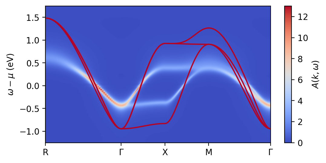
That’s it. Now you can look at the output:

if kslice:
    fig, ax = plt.subplots(1, figsize=(3,3), dpi=200)

    pcb.plot_kslice(fig, ax, alatt_k_w, tb_data, freq_dict, w90_dict['n_orb'], tb_config,
                    tb=config['tb'], alatt=config['alatt'], quarter=0, **plot_config)

else:
    fig, ax = plt.subplots(1, figsize=(6,3), dpi=200)

    pcb.plot_bands(fig, ax, alatt_k_w, tb_data, freq_dict, w90_dict['n_orb'], dft_mu=0.,
                   tb=config['tb'], alatt=config['alatt'], qp_bands=config['qp_bands'], **plot_config)

    ax.set_ylim(-1.25,1.75)

---