Single-Orbital Hubbard Model (Bethe Lattice)

Script: examples/Bethe_1orb.py

In this example we will address the most canonical example of calculation for local quantum embedding theories that is solving the single orbital Hubbard model on the Bethe lattice (semicircular DOS, half-bandwidth \(D = 1\)) performing a sweep over the Hubbard \(U\). In this calculation we will enforce spin SU(2) symmetry and we will track the quasiparticle weight \(Z\) as a function of \(U\), revealing the Mott metal-insulator transition.

Setup

We start from importing the necessary modules:

import numpy as np
import matplotlib.pyplot as plt
from gem.lattice import Lattice
from gem.fragment import Fragment
from gem.solvers.simple_ed import SimpleED

We sample the semicircular DOS on a fine energy mesh, we use to build the dispersion array and relative weights, and we use them to initialize the lattice object:

# 1 orbital x 2 spins, B=3 bath orbitals per spin
nimp, B = 2, 3
nbath, ntot = nimp * B, nimp + nimp * B

# semicircular DOS on a fine energy mesh
e_list = np.linspace(-1, 1, 5001)
wks = np.sqrt(1 - e_list**2); wks /= wks.sum()
eks = np.array([np.kron([[e]], np.eye(2)) for e in e_list])

lattice = Lattice(eks, wk_list=wks)

Self-consistency loop

For each value of \(U\) the embedding local Hamiltonian is built and a solver object is created. Those will be the inputs of the Fragment object that and the ghost-GA equations are iterated to convergence:

U = 2.5
eloc = np.diag([-U/2, -U/2])
Utensor = np.zeros((nimp,)*4)
Utensor[0, 0, 1, 1] = Utensor[1, 1, 0, 0] = U

solver   = SimpleED(ntot, use_Ntot=True, use_Sz=True,
                    N_sector=ntot//2, Sz_sector=0,
                    dtype=np.complex128)
fragment = Fragment(nimp, nbath, eloc, Utensor, solver)

mu, T, mix, tol = 0.0, 0.0, 0.5, 1e-5
for it in range(100):
    lattice.solve_qp([fragment], T=T)
    fragment.update_hybridization(T=T)
    fragment.impose_spin_SU2_symmetry()
    fragment.solve_impurity(mu, T=T, num_eig=10)

    Lambda_old, R_old = fragment.Lambda.copy(), fragment.R.copy()
    fragment.update_self_energy(T=T)
    fragment.impose_spin_SU2_symmetry()

    diff = max(np.abs(fragment.Lambda - Lambda_old).max(),
               np.abs(fragment.R      - R_old     ).max())
    fragment.Lambda = (1 - mix)*fragment.Lambda + mix*Lambda_old
    fragment.R      = (1 - mix)*fragment.R      + mix*R_old
    fragment.impose_spin_SU2_symmetry()
    if diff < tol and it > 2:
        break

Z = fragment.compute_Z()

Note that, since we are working with a paramagnetic solution, the local Hamiltonian is spin-symmetric and the solver is set to work in the subspace of fixed total particle number and magnetization via the use_Ntot and use_Sz flags and indicating the corresponding sectors N_sector=ntot//2 and Sz_sector=0. The call to impose_spin_SU2_symmetry after each step enforces that the \(\uparrow\) and \(\downarrow\) sectors remain identical, keeping the solution in the paramagnetic state throughout the sweep. When performing single site calculations, the quasiparticle weight can be computed from local self-energy and the fragment object provides a method compute_Z to do so.

Results

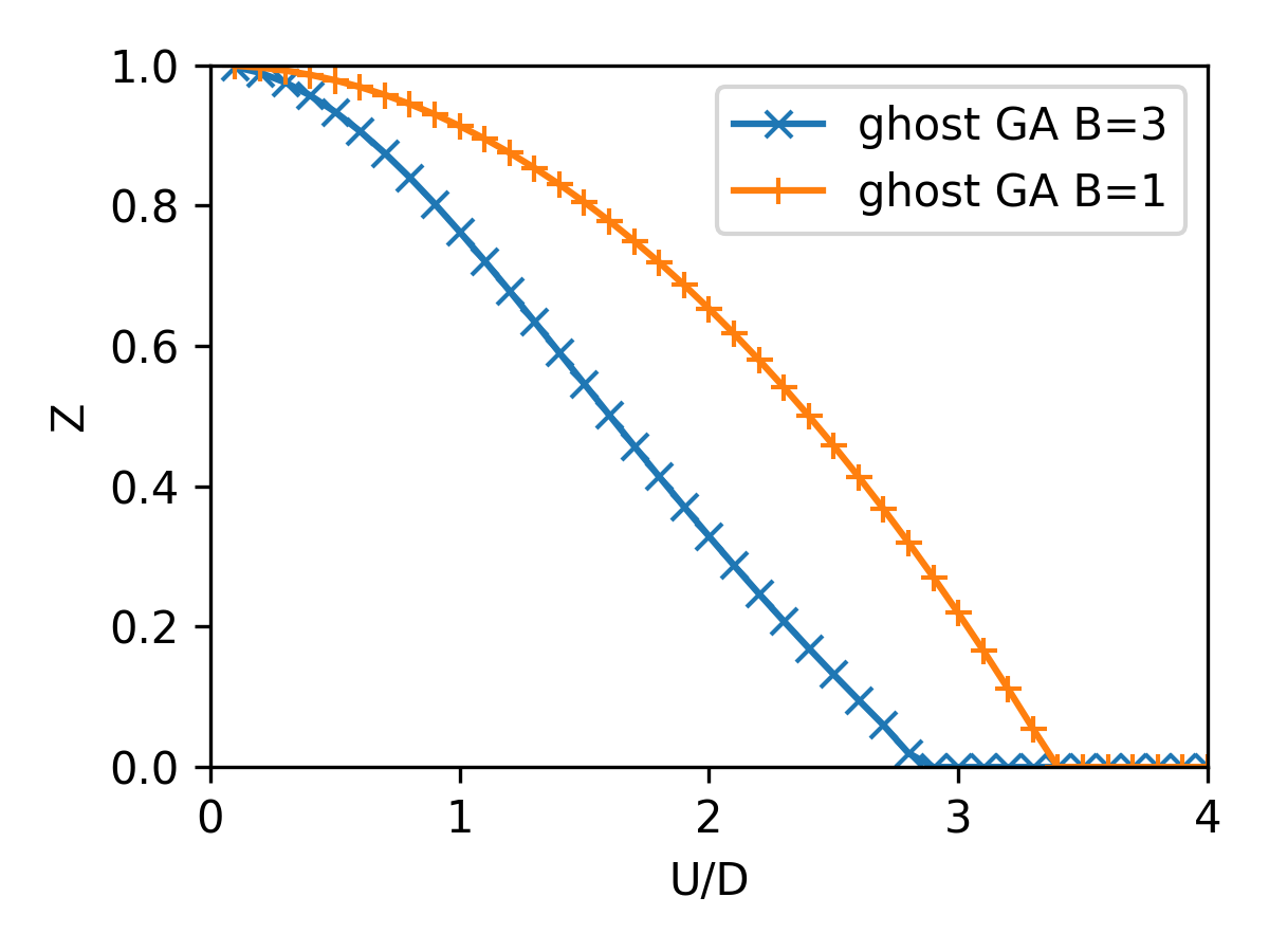
Performing the sweep over \(U\) and plotting the resulting \(Z(U)\) curve, we can clearly see the Mott transition and the difference in critical interaction between the standard GA (\(B=1\), orange) and ghost GA (\(B > 1\) , in this case \(B=3\), blue ):

Additionally, we can check how the spectral function evolves across the transition, by plotting the imaginary part of the local lattice Green’s function. The lattice Green’s function is computed from the lattice object via the method get_G_loc directly on the real-frequency axis passing an array of frequencies and a small imaginary broadening:

w_list = np.linspace(-3, 3, 500)
G_loc_w = lattice.get_G_loc(w_list, [fragment], eps=1e-2)[0]

The resulting spectral functions for the different values of \(U\) are shown in the following figure:

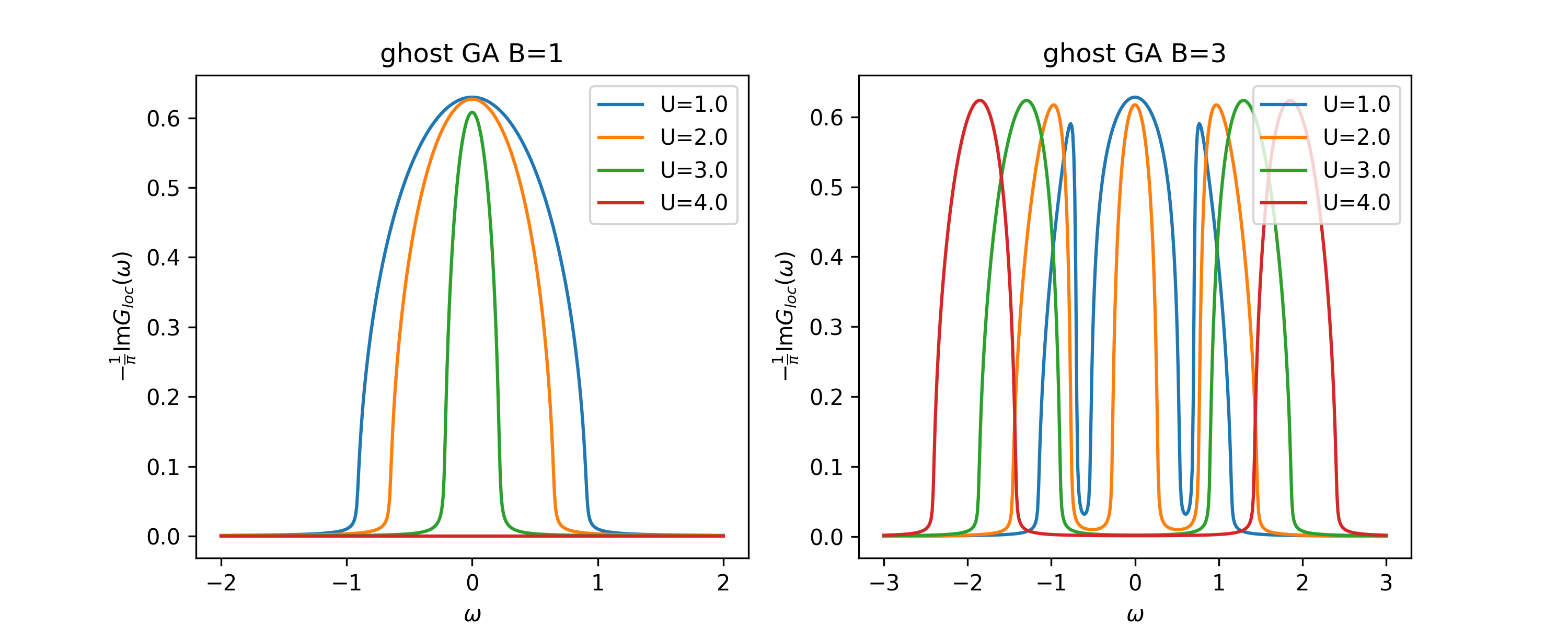
The disappearence of the quasiparticle peak after the Mott transition is clearly visible for both \(B=1\) and \(B=3\). Although, only the latter is able to capture the Mott gap opening at the transition.