Square Lattice — AFM Phase Diagram (Finite Temperature)
Script: examples/Square_1orb_2frag_phase.py
Plotting: examples/plot_phase_B3.py
This example maps out the finite-temperature antiferromagnetic (AFM) phase diagram of the single-orbital Hubbard model on the square lattice. For each value of \(U\), the staggered magnetisation \(|m|\) is tracked as a function of temperature \(T\), sweeping from low to high \(T\) on a uniform grid. The result is a dataset from which the critical temperature \(T_c(U)\) can be extracted, tracing the boundary between the AFM ordered phase and the paramagnetic phase in the \((U, T)\) plane.
Setup
We import the necessary modules:
import numpy as np
from gem.fragment import Fragment
from gem.lattice  import Lattice
from gem.solvers.simple_ed import SimpleED
import h5py
The square-lattice setup follows the same structure as Square Lattice — Antiferromagnetic Order (T = 0):
B     = 3
nimp  = 2
nbath = nimp * B
ntot  = nimp + nbath

Nk = 200
Kx = np.linspace(-np.pi, np.pi, Nk, endpoint=False)
Ky = np.linspace(-np.pi, np.pi, Nk, endpoint=False)
t  = 0.25

ek_list = []
for kx in Kx:
    for ky in Ky:
        gamma_k = -t * (1.0
                    + np.exp(-1j * (kx + ky))
                    + np.exp(-1j * ky)
                    + np.exp(-1j * kx))
        Hk_spinless = np.array([[0.0, gamma_k],
                                [gamma_k.conj(), 0.0]], dtype=np.complex128)
        ek_list.append(np.kron(Hk_spinless, np.eye(2)))

eks = np.array(ek_list)
wks = np.ones(len(ek_list)) / len(ek_list)
lattice = Lattice(eks, wk_list=wks)
The interaction and temperature grids are:
U_list = np.array([0.5, 1.5, 2.0, 2.5, 4.0])
T_list = np.linspace(0, 0.10, 51)

mag_grid = np.zeros((len(U_list), len(T_list)))
Results are accumulated in mag_grid[iU, iT] = \(|m_A|\), the
staggered order parameter on sublattice A.
Initial guess
The bath parameters are initialised with a staggered spin-splitting to seed the AFM solution:
L_t0  = np.kron(np.tanh(np.diag(np.linspace(-1, 1, B+1, endpoint=False)[1:])),
                np.eye(2))
L_t0A = L_t0 + 1e-1 * np.kron(np.eye(B), np.diag([1.0, -1.0]))
L_t0B = -L_t0A
R_t0  = np.kron(np.ones((B, 1)) / np.sqrt(B), np.eye(2))
L_t0 provides a bath with spread energy levels via a tanh profile.
The small perturbation 1e-1 * diag([1, -1]) introduces opposite
spin-splittings on the two sublattices A and B, breaking the symmetry
and stabilising the AFM solution from the first iteration.
Seeding AFM order
In addition to the asymmetric initial guess, a weak symmetry-breaking
field bfield = 1e-2 is applied to the local levels only at the
lowest temperature point for the first few self-consistency
iterations:
if iT == 0 and it < 3:
    fragmentA.eloc = eloc + bfield * np.diag([-1,  1])
    fragmentB.eloc = eloc - bfield * np.diag([-1,  1])
else:
    fragmentA.eloc = eloc.copy()
    fragmentB.eloc = eloc.copy()
This is sufficient because the warm-start strategy (see below) propagates the ordered solution from one temperature to the next without requiring a bias field at each \(T\).
Warm-starting across temperatures
The converged variational parameters \(R\), \(\Lambda\), \(D\), and \(\Lambda_c\) from one temperature point are used as the initial guess for the next. This dramatically reduces the number of iterations needed near the transition and allows the ordered solution to survive into the high-\(T\) regime until it is destabilised by thermal fluctuations:
Lambda_A, R_A = L_t0A.copy(), R_t0.copy()
Lambda_c_A, D_A = L_t0A.copy(), R_t0.copy()
Lambda_B, R_B = L_t0B.copy(), R_t0.copy()
Lambda_c_B, D_B = L_t0B.copy(), R_t0.copy()

for iT, T in enumerate(T_list):
    fragmentA = Fragment(..., Lambda=Lambda_A, R=R_A,
                         Lambda_c=Lambda_c_A, D=D_A)
    fragmentB = Fragment(..., Lambda=Lambda_B, R=R_B,
                         Lambda_c=Lambda_c_B, D=D_B)

    # ... self-consistency loop ...

    Lambda_A, R_A = fragmentA.Lambda.copy(), fragmentA.R.copy()
    Lambda_c_A, D_A = fragmentA.Lambda_c.copy(), fragmentA.D.copy()
    Lambda_B, R_B = fragmentB.Lambda.copy(), fragmentB.R.copy()
    Lambda_c_B, D_B = fragmentB.Lambda_c.copy(), fragmentB.D.copy()
Enforcing magnetisation along the z-axis
To ensure that the magnetisation is purely along the z-axis the spin-off-diagonal elements of \(R\), \(\Lambda\), \(D\), and \(\Lambda_c\) are zeroed at every iteration:
for fragment in [fragmentA, fragmentB]:
    fragment.R[::2, 1::2] = 0.0;  fragment.R[1::2, ::2] = 0.0
    fragment.Lambda[::2, 1::2] = 0.0;  fragment.Lambda[1::2, ::2] = 0.0
    fragment.D[::2, 1::2] = 0.0;  fragment.D[1::2, ::2] = 0.0
    fragment.Lambda_c[::2, 1::2] = 0.0;  fragment.Lambda_c[1::2, ::2] = 0.0
The \(R\) and \(\Lambda\) projections are applied before
lattice.solve_qp; the \(D\) and \(\Lambda_c\) projections are
applied after update_hybridization.
Convergence criterion
The self-consistency loop is considered converged when the combined residual:
diff = max(diff_LR, 10 * diff_A, 10 * diff_B)
falls below tol = 1e-3. Here diff_LR is the maximum change in
\(\Lambda\) and \(|R|\) across both fragments, while diff_A
and diff_B are the changes in the staggered magnetisation on each
sublattice. The factor of 10 gives extra weight to magnetisation
convergence, which is the physically relevant order parameter.
Storing results
After each \(U\) is completed, the full one-body density matrix, the variational parameters \(R\) and \(\Lambda\), and the quasiparticle weight \(Z\) for both fragments are written to an HDF5 file, one group per \(U\) value:
with h5py.File(f'data_Square_1orb_2frag_B{B}_phase.h5', 'a') as h5f:
    grp = h5f.create_group(f'U{U:.2f}_B{B}')
    grp.create_dataset('T_list',   data=T_list)
    grp.create_dataset('denMat_A', data=arr_denMat_A)  # shape (nT, nimp, nimp)
    grp.create_dataset('denMat_B', data=arr_denMat_B)
    grp.create_dataset('R_A',      data=arr_R_A)       # shape (nT, nbath, nimp)
    grp.create_dataset('R_B',      data=arr_R_B)
    grp.create_dataset('Lambda_A', data=arr_Lambda_A)  # shape (nT, nbath, nbath)
    grp.create_dataset('Lambda_B', data=arr_Lambda_B)
    grp.create_dataset('Z_A',      data=arr_Z_A)       # shape (nT, nimp, nimp)
    grp.create_dataset('Z_B',      data=arr_Z_B)
Each group is flushed to disk as soon as the \(U\) sweep completes,
so partial runs are not lost if the script is interrupted. The file is
opened in append mode ('a'), which lets successive runs with
different \(U\) values accumulate in the same file without
overwriting completed groups.
Mean-field criticality fit
The companion script plot_phase_B3.py reads the HDF5 file and fits
the mean-field order-parameter form
to the magnetisation near each critical temperature. The fit is restricted to the critical region, excluding both the low-\(T\) saturated regime and the high-\(T\) noise floor. It produces three output figures:
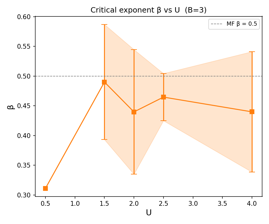
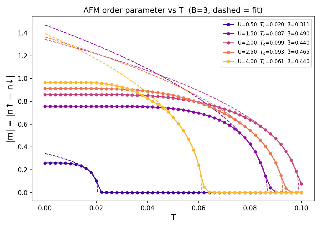
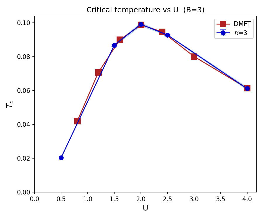
B3_mag_vs_T.png— \(|m(T)|\) for all \(U\) values with the MF fits overlaid as dashed lines.B3_Tc_vs_U.png— the critical temperature \(T_c(U)\) with fit uncertainties shown as error bars and a shaded ±1σ band.B3_beta_vs_U.png— the fitted exponent \(\beta(U)\) with error bars and the mean-field reference \(\beta = 1/2\).
Results
The order parameter \(|m|\) as a function of temperature for different values of \(U\) is shown below. The critical temperature \(T_c\) increases and reaches a maximum for \(U \approx 2.0\) across the range studied.
The critical temperatures \(T_c(U)\) are shown below together with data extracted from DMFT. We can see clearly that already \(B=3\) reproduces faithfully the AFM dome of DMFT extracted from Phys. Rev. B 83, 085102 (2011).
The fitted exponent \(\beta(U)\) are shown below. The extracted values are consistent with the mean-field value \(\beta = 1/2\), apart from the small interaction \(U=0.5\) where there are few points to fit. This is expected for a ghost-GA calculation since it reproduces the DMFT critical behavior