Single-Orbital Hubbard Model (Triangular Lattice via TRIQS)
Script: examples/Triangular_TRIQS_1orb.py
This example solves the single-orbital Hubbard model on the two-dimensional
triangular lattice, a canonical frustrated-geometry system.
The tight-binding model is constructed with TRIQS’s TBLattice class,
which generates the Hamiltonian \(H(\mathbf{k})\) on an explicit
Brillouin-zone mesh.
As in the Bethe-lattice example (see Single-Orbital Hubbard Model (Bethe Lattice)), we track the
quasiparticle weight \(Z\) as a function of the Hubbard interaction
\(U\) at half filling, using spin SU(2) symmetry to keep the solution
paramagnetic throughout the sweep.
Setup
We import the standard GEM modules together with TRIQS’s tight-binding class:
import numpy as np
import matplotlib.pyplot as plt
from triqs.lattice.tight_binding import TBLattice
from gem.fragment import Fragment
from gem.lattice import Lattice
from gem.solvers.simple_ed import SimpleED
The triangular lattice is defined by two primitive vectors in Cartesian coordinates and nearest-neighbor hopping amplitude \(t = 1\):
a1 = np.array([1.0, 0.0, 0.0])
a2 = np.array([0.5, np.sqrt(3.0) / 2.0, 0.0])
t  = 1.0

H_t = TBLattice(
    units=[a1, a2],
    hoppings={
        (+1,  0): [[-t]],
        (-1,  0): [[-t]],
        ( 0, +1): [[-t]],
        ( 0, -1): [[-t]],
        (+1, -1): [[-t]],
        (-1, +1): [[-t]],
    }
)
A uniform \(64 \times 64\) k-mesh is generated from the TBLattice
object and the Hamiltonian is evaluated at each k-point.
The spin degree of freedom is added by tensoring with the
\(2 \times 2\) identity matrix so that each orbital carries two spins:
Nk    = 64
kmesh = H_t.get_kmesh((Nk, Nk, 1))
kpts  = np.array(list(kmesh.values()))

# shape: (Nk^2, 2, 2)  — one 2x2 block per k-point (1 orbital x 2 spins)
Hk_list = np.array([np.kron(H_t.fourier(k), np.eye(2)) for k in kpts])

lattice = Lattice(Hk_list)
The fragment is set up with \(B = 3\) bath sites per spin, giving
nimp = 2 impurity levels (one per spin) and nbath = 6 bath levels:
nimp, B   = 2, 3
nbath     = nimp * B
ntot      = nimp + nbath
Self-consistency loop
For each value of \(U\) the local Hamiltonian and interaction tensor are
built, a SimpleED solver is instantiated, and the ghost-GA equations are
iterated to convergence.
Because the triangular lattice is frustrated and the chemical potential can
drift away from half filling during the self-consistency, the code fits
\(\mu\) on the fly whenever the impurity filling deviates from the target
\(n = 1\):
fit_mu   = True
n_target = 1.0          # half filling: one electron per site
mu       = 0.0

for U in U_list:
    eloc         = np.diag([-U/2, -U/2])
    Utensor      = np.zeros((nimp,)*4)
    Utensor[0, 0, 1, 1] = Utensor[1, 1, 0, 0] = U

    solver   = SimpleED(ntot, use_Ntot=True, use_Sz=True,
                        N_sector=ntot//2, Sz_sector=0,
                        dtype=np.complex128)
    fragment = Fragment(nimp, nbath, eloc, Utensor, solver,
                        Lambda=Lambda0, R=R0, verbose=2)

    for it in range(itmax):
        lattice.solve_qp([fragment], T=T)
        fragment.update_hybridization(T=T)
        fragment.impose_spin_SU2_symmetry()

        fragment.solve_impurity(mu, T=T, num_eig=10, spin_pen=spin_pen)

        # adjust mu to maintain half filling
        if abs(fragment.nfill - n_target) > 1e-3 and fit_mu:
            mu = lattice.fit_mu(n_target, [fragment], T=T,
                                mu_old=mu, mode='imp', ntol=1e-4)

        Lambda_old, R_old = fragment.Lambda.copy(), fragment.R.copy()
        fragment.update_self_energy(T=T)
        fragment.impose_spin_SU2_symmetry()

        # convergence check in the eigenframe of Lambda
        L_eval_new, UL_new = np.linalg.eigh(fragment.Lambda[::2, ::2])
        L_eval_old, UL_old = np.linalg.eigh(Lambda_old[::2, ::2])
        diff = max(
            np.abs(np.abs(UL_old @ R_old[::2, ::2])
                   - np.abs(UL_new @ fragment.R[::2, ::2])).max(),
            np.abs(L_eval_new - L_eval_old).max(),
        )

        fragment.Lambda = (1 - mix)*fragment.Lambda + mix*Lambda_old
        fragment.R      = (1 - mix)*fragment.R      + mix*R_old
        fragment.impose_spin_SU2_symmetry()

        if diff < tol and it > 2:
            break

    Z_list.append(fragment.compute_Z()[0, 0].real)
    # warm-start next U from current converged solution
    Lambda0, R0 = fragment.Lambda.copy(), fragment.R.copy()
Once the lattice information is encoded in the lattice object, the self-consistency loop is similar to the Bethe-lattice case.
The absence of particle-hole symmetry in this case require the chemical potential to be adjusted on the fly to maintain half filling.
We do that by calling the fit_mu method of the lattice object whenever the impurity filling deviates from the target by more than a certain threshold (e.g., 0.001).
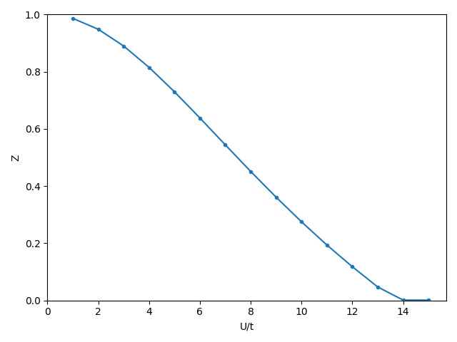
Results
Plotting the quasiparticle weight \(Z\) as a function of \(U\) reveals the Mott metal-insulator transition on the triangular lattice:
plt.figure()
plt.plot(U_list, Z_list,marker='.')
plt.ylabel('Z')
plt.xlabel('U/t')
plt.xlim(0,None)
plt.ylim(0,1)
plt.tight_layout()
plt.savefig(f'trZ_vs_U_B{B}.png', dpi=100)
plt.show()
As \(U\) increases from zero the quasiparticle weight decreases continuously from 1 toward 0, marking the gradual loss of coherence before the insulating state is reached. The frustrated geometry of the triangular lattice shifts the critical interaction to a larger value compared to the Bethe-lattice result, and the ghost-GA treatment (\(B = 3\)) captures the correct shape of the \(Z(U)\) curve more accurately than the standard Gutzwiller approximation (\(B = 1\)).