Square Lattice — Antiferromagnetic Order (T = 0)

Script: examples/Square_1orb_2frag.py

In this example we study the single-orbital Hubbard model on the square lattice at zero temperature and look for antiferromagnetic (AFM) order. The square lattice has a nested Fermi surface, which makes it especially susceptible to spin-density-wave instabilities, and therefore a natural test case for broken-symmetry ghost-GA calculations.

A two-site unit cell is used, with one fragment per sublattice (A and B). The two fragments are allowed to develop opposite spin polarisations by not imposing spin SU(2) symmetry. A sweep over the Hubbard \(U\) is performed and the double occupancy \(\langle n_\uparrow n_\downarrow \rangle\) and staggered magnetisation \(m = n_\uparrow - n_\downarrow\) are extracted from each converged solution.

Setup

We start by importing the necessary modules:

import numpy as np
from gem.fragment import Fragment
from gem.lattice import Lattice
from gem.solvers.simple_ed import SimpleED

We consider one orbital with two spin components (nimp = 2) and B ghost orbitals per spin channel (B = 1 being GA and B > 1 being ghost GA):

B = 1
nimp = 2
nbath = nimp * B
ntot  = nimp + nbath

The square-lattice Brillouin zone is sampled on a uniform \(100 \times 100\) k-grid. We set the nearest-neighbour hopping amplitude to \(t = 0.25\) so that the non-interacting half-bandwidth is the unit of energy. The two-site unit cell gives an off-diagonal hopping \(\gamma_\mathbf{k}\), and the single-particle Hamiltonian is built in the combined (site, spin) basis via a Kronecker product:

Nk = 100
Kx = np.linspace(-np.pi, np.pi, Nk, endpoint=False)
Ky = np.linspace(-np.pi, np.pi, Nk, endpoint=False)
t  = 0.25

ek_list = []
for kx in Kx:
    for ky in Ky:
        gamma_k = -t * (1.0
                    + np.exp(-1j * (kx + ky))
                    + np.exp(-1j * ky)
                    + np.exp(-1j * kx))
        Hk_spinless = np.array([[0.0, gamma_k],
                                [gamma_k.conj(), 0.0]], dtype=np.complex128)
        ek_list.append(np.kron(Hk_spinless, np.eye(2)))

eks = np.array(ek_list)
wks = np.ones(len(ek_list)) / len(ek_list)
lattice = Lattice(eks, wk_list=wks)

Self-consistency loop

For each value of \(U\) a pair of fragment objects is created, one per sublattice, sharing the same local Hamiltonian, both local energy via the matrix eloc and the interaction tensor Utensor which encodes the on-site Hubbard repulsion between spin-up and spin-down electrons, but they will carry independent variational parameters \(\mathcal{R}\), \(\Lambda\), \(\mathcal{D}\) and \(\Lambda_c\). Since the Hamiltonian preserve the total particle number and the z-component of the total spin, the impurity solvers are initialized to take advantage of the symmetry sectors at fixed \(N_\mathrm{tot}\) and \(S_z\) via the flags use_Ntot and use_Sz:

eloc = np.zeros((nimp, nimp))
eloc[0, 0] = -U / 2.
eloc[1, 1] = -U / 2.

Utensor = np.zeros((nimp, nimp, nimp, nimp))
Utensor[0, 0, 1, 1] = U
Utensor[1, 1, 0, 0] = U

edsolverA = SimpleED(ntot, use_Ntot=True, use_Sz=True,
                     N_sector=ntot//2, dtype=np.complex128)
edsolverB = SimpleED(ntot, use_Ntot=True, use_Sz=True,
                     N_sector=ntot//2, dtype=np.complex128)
fragmentA = Fragment(nimp, nbath, eloc, Utensor, edsolverA,
                     Lambda=Lambda0, R=R0)
fragmentB = Fragment(nimp, nbath, eloc, Utensor, edsolverB,
                     Lambda=Lambda0, R=R0)

The ghost-GA self-consistency loop is then run for up to itmax iterations with a linear mixing mix between the new and old variational parameters:

for it in range(itmax):
    lattice.solve_qp([fragmentA, fragmentB], T=T)

    fragmentA.update_hybridization(T=T)
    fragmentB.update_hybridization(T=T)

    # seeding AFM order... See below for details

    fragmentA.solve_impurity(mu, T=T)
    fragmentB.solve_impurity(mu, T=T)

    Lambda_old_A, R_old_A = fragmentA.Lambda.copy(), fragmentA.R.copy()
    Lambda_old_B, R_old_B = fragmentB.Lambda.copy(), fragmentB.R.copy()

    fragmentA.update_self_energy(T=T)
    fragmentB.update_self_energy(T=T)

    diff = max(
        np.abs(fragmentA.Lambda - Lambda_old_A).max(),
        np.abs(fragmentA.R      - R_old_A     ).max(),
        np.abs(fragmentB.Lambda - Lambda_old_B).max(),
        np.abs(fragmentB.R      - R_old_B     ).max(),
    )
    fragmentA.Lambda = (1 - mix)*fragmentA.Lambda + mix*Lambda_old_A
    fragmentA.R      = (1 - mix)*fragmentA.R      + mix*R_old_A
    fragmentB.Lambda = (1 - mix)*fragmentB.Lambda + mix*Lambda_old_B
    fragmentB.R      = (1 - mix)*fragmentB.R      + mix*R_old_B

    if diff < tol and it > 2:
        break

Seeding AFM order

A self-consistency iteration will in principle be satisfied by the paramagnetic solution (equal spin populations on both sublattices) even when the ordered phase is the true ground state. To bias the iteration towards the AFM solution, a small symmetry-breaking Zeeman field with opposite sign on the two sublattices is applied to the on-site energies during the first few iterations:

if it < 3:
    fragmentA.eloc = eloc + bfield * np.diag([-1,  1])
    fragmentB.eloc = eloc - bfield * np.diag([-1,  1])
else:
    fragmentA.eloc = eloc.copy()
    fragmentB.eloc = eloc.copy()

Once the field is removed, if the system is in the ordered phase the solution remains magnetised because the two fragments have already developed a finite \(R\) and \(\Lambda\) asymmetry. In the paramagnetic phase the solution relaxes back to \(m = 0\).

Extracting the results

After convergence, the double occupancy is computed from each fragment, and the magnetisation on each sublattice is read from the impurity block of the converged one-body density matrix:

docc_A = fragmentA.compute_docc()
docc_B = fragmentB.compute_docc()

dm_A = fragmentA.denMat[:nimp, :nimp].real # local impurity density matrix of fragment A
dm_B = fragmentB.denMat[:nimp, :nimp].real # local impurity density matrix of fragment B
mA = dm_A[0, 0] - dm_A[1, 1]   # n_↑ - n_↓ on sublattice A
mB = dm_B[0, 0] - dm_B[1, 1]   # n_↑ - n_↓ on sublattice B

In the ordered phase \(m_A = -m_B \neq 0\) by symmetry of the two-sublattice unit cell.

Results

The following figures show the double occupancy \(\langle n_\uparrow n_\downarrow \rangle\) and the staggered magnetisation \(m\) as a function of \(U\) for the square-lattice Hubbard model at zero temperature.

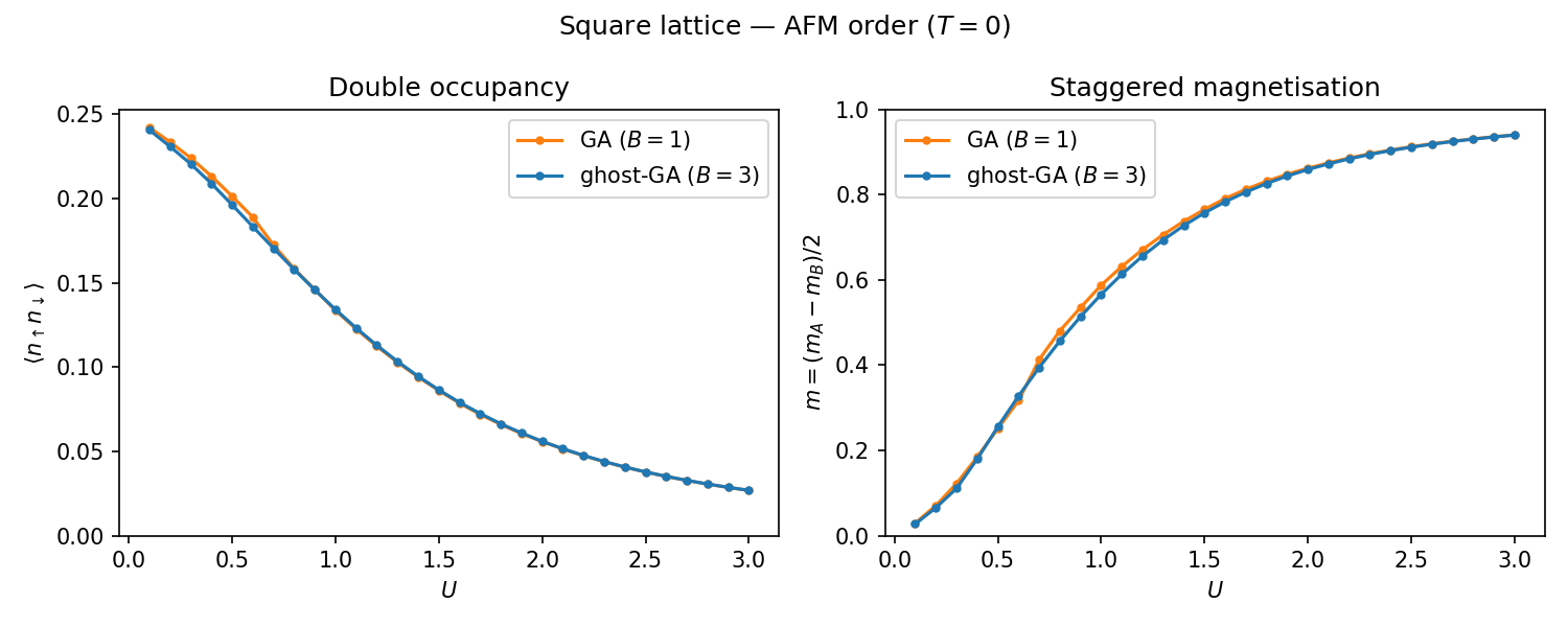
The double occupancy \(\langle n_\uparrow n_\downarrow \rangle\) decreases with increasing \(U\) as the system becomes more correlated and the staggered magnetisation \(m\) increases monotonically with increasing \(U\).

At small \(U\) the system is a paramagnet (\(m = 0\)), while above a critical \(U_c\) a finite staggered magnetisation develops. The onset of magnetic order coincides with a reduction of the quasiparticle weight \(Z\), reflecting the increased effective mass of carriers in the AFM phase.