E1 — Thermodynamics of the Hubbard Model on the Bethe Lattice
Script: examples/E1/Bethe_1orb.py
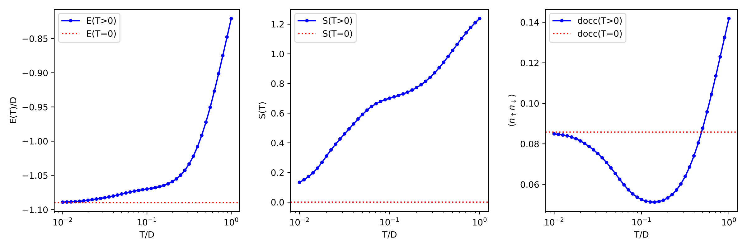
This example follows the half-filled single-orbital Hubbard model on the Bethe lattice (semicircular DOS, half-bandwidth \(D = 1\)) at fixed \(U = 2\) along a temperature scan, and extracts some of the thermodynamic quantities that the finite-temperature formulation gives access to: the total energy \(E(T)\), the entropy per site \(S(T)\), and the double occupancy \(\langle n_\uparrow n_\downarrow \rangle (T)\). The same quantities are discussed in Ref. [2].
Setup
The dimensions are fixed by one orbital with two spins and \(B = 3\) ghost
levels per spin-orbital, so the embedding problem has ntot = 8 levels:
import numpy as np
from gem.fragment import Fragment
from gem.lattice import Lattice
from gem.solvers.simple_ed import SimpleED

B, nimp = 3, 2
nbath = nimp * B
ntot  = nimp + nbath

U, mu = 2.0, 1.0
Tlist = np.hstack((np.array([0]),
                   np.logspace(np.log10(1e-3), np.log10(1), 31)))

itmax, tol, Tsmearing = 100, 1e-5, 1e-3
The semicircular density of states is sampled on a fine energy mesh and enters
the Lattice as the dispersion together with its weights:
e_list = np.linspace(-1, 1, 5001)
wks = np.sqrt(1 - e_list**2)
wks /= np.sum(wks)
eks = e_list[:, None, None] * np.eye(2, dtype=np.complex128)

lattice = Lattice(eks, wk_list=wks)
The local Hamiltonian is a plain Hubbard \(U\), and the chemical potential
mu = U/2 puts the model at half filling:
eloc = np.zeros((nimp, nimp))
Utensor = np.zeros((nimp, nimp, nimp, nimp))
Utensor[0,0,1,1] = U
Utensor[1,1,0,0] = U
Because the scan runs up to \(T = 1\), no particle-number or \(S_z\)
sector can be fixed: the thermal averages must be taken over the whole Fock
space, hence N_sector=None, Sz_sector=None. The fragment is created once and
reused along the whole temperature scan, so each temperature warm-starts from
the parameters converged at the previous one:
edsolver = SimpleED(ntot, use_Ntot=True, use_Sz=True,
                    N_sector=None, Sz_sector=None, dtype=np.float64)

fragment = Fragment(nimp, nbath, eloc, Utensor, edsolver,
                    Lambda=None, R=None, verbose=2)
Self-consistency loop
For every temperature in Tlist the four steps of the cycle are iterated
until the self-energy parameters stop moving. Convergence is measured on a
gauge-invariant combination — the eigenvalues of \(\Lambda\) and the moduli
of \(R\) rotated into its eigenbasis — because \(R\) and \(\Lambda\)
are only defined up to the gauge freedom of the ghost sector:
def check_convergence(R_new, L_new, R_old, L_old):
    L_eval_new, UL_new = np.linalg.eigh(L_new[::2,::2])
    L_eval_old, UL_old = np.linalg.eigh(L_old[::2,::2])
    diff_R = np.abs(np.abs(UL_old @ R_old[::2,::2])
                    - np.abs(UL_new @ R_new[::2,::2])).max()
    diff_Lambda = np.abs(L_eval_new - L_eval_old).max()
    return max(diff_R, diff_Lambda)

for T in Tlist:
    for it in range(itmax):
        lattice.solve_qp([fragment], T=T, Tsmearing=Tsmearing)
        fragment.update_hybridization(T=T, use_Sz=True)
        fragment.solve_impurity(mu, T=T)
        Lambda_old, R_old = fragment.Lambda.copy(), fragment.R.copy()
        fragment.update_self_energy(T=T, use_Sz=True)

        diff = check_convergence(fragment.R, fragment.Lambda, R_old, Lambda_old)
        if (diff < tol and it > 2) or it == itmax - 1:
            break
use_Sz=True keeps \(S_z\) a good quantum number in the update, which
keeps the solution paramagnetic. Tsmearing only acts on the \(T = 0\)
point of the scan, where it regularises the Fermi function of the quasiparticle
problem.
Observables
Once converged, the double occupancy is read off the local interaction energy,
and the total energy is the sum of the kinetic and the impurity contributions.
The entropy follows from the free-energy functional of Eq. (11),
evaluated by compute_functional(), through
\(S = (E - \mathcal{L}_\beta)/T\):
docc = fragment.E2loc / U
ekin = lattice.compute_ekin([fragment], T=T, Tsmearing=Tsmearing)
eimp = fragment.compute_energy()
etot = (eimp + ekin).real

L = lattice.compute_functional([fragment], T=T, Tsmearing=Tsmearing).real
S = (etot - L) / T if T > 0 else 0.0
The scan is written to Tlist.dat, Elist.dat, Slist.dat and
docclist.dat as the results are plotted in the following figure, with the
\(T = 0\) value of each quantity drawn as a
horizontal reference line.
Results