E2 — Antiferromagnetism on the Square Lattice and its Critical Temperature
Script: examples/E2/Square_1orb_2frag_phase.py
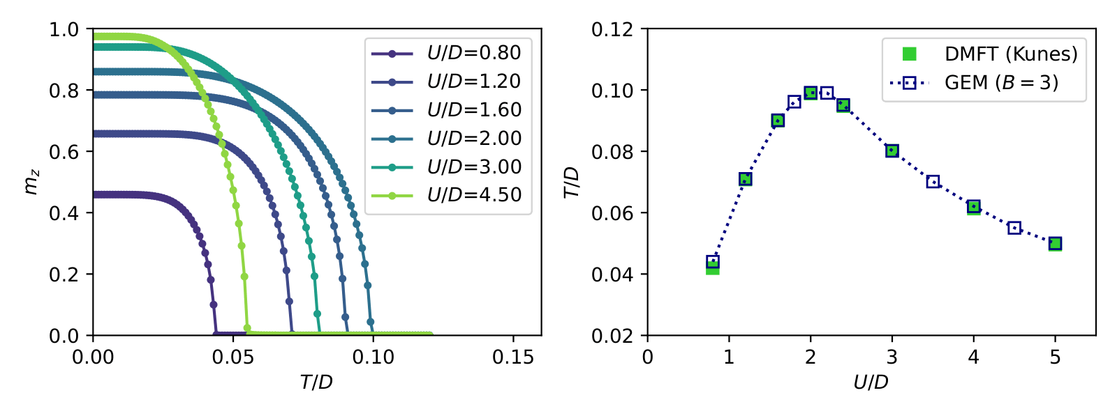
This example addresses the half-filled single-orbital Hubbard model on the square lattice, described with two fragments — the A and B sublattices of the Néel unit cell — so that antiferromagnetic order can develop. A temperature scan at fixed \(U\) tracks the staggered magnetisation \(m = \frac{1}{2}(m_A - m_B)\) across the ordering transition.
Setup
Each sublattice carries one orbital with two spins and \(B = 3\) ghost
levels per spin-orbital. The temperature is scanned at one value of \(U\)
per run; the results are accumulated in a group U<U>_B<B> of an HDF5 file,
so repeated runs at different \(U\) build up the phase diagram in the same
file:
import numpy as np
import h5py
from gem.fragment import Fragment
from gem.lattice import Lattice
from gem.solvers.simple_ed import SimpleED

nimp, B = 2, 3
nbath = nimp * B
ntot  = nimp + nbath

U, mu, t, bfield = 0.8, 0.4, 0.25, 1e-2
T_list = np.linspace(0.0, 0.10, 51)

itmax, tol, mix, move_pen, Tsmearing = 200, 1e-3, 0.05, 1e-8, 1e-3
h5_file = f'data_Square_1orb_2frag_B{B}_phase.h5'
The dispersion is generated with TRIQS’ TBLattice, in the two-site unit cell
that alternates the sublattices: A at \((0,0)\), B at \((1,0)\), and
primitive vectors along the diagonals:
from triqs.lattice.tight_binding import TBLattice

a1, a2 = np.array([1.0, 1.0, 0.0]), np.array([1.0, -1.0, 0.0])
H_t = TBLattice(
    units=[a1, a2],
    hoppings={( 0,  0): [[0, -t], [-t, 0]],
              (-1, -1): [[0, -t], [ 0, 0]], ( 1,  1): [[0,  0], [-t, 0]],
              ( 0, -1): [[0, -t], [ 0, 0]], ( 0,  1): [[0,  0], [-t, 0]],
              (-1,  0): [[0, -t], [ 0, 0]], ( 1,  0): [[0,  0], [-t, 0]]},
    orbital_positions=[(0, 0, 0), (1, 0, 0)], orbital_names=['A', 'B'],
)

Nk = 200
kmesh = H_t.get_kmesh((Nk, Nk, 1))
kpts_cart = np.array(list(kmesh.values()))
recip = np.array(kmesh.bz.units)
kpts  = kpts_cart @ np.linalg.inv(recip)

eks = np.array([np.kron(H_t.fourier(k), np.eye(2)) for k in kpts])
lattice = Lattice(eks)
Each \(H(k)\) is a \(4 \times 4\) matrix — two sublattices times two spins — matching the total number of impurity levels of the two fragments. The weights are left to their default, which is the uniform \(1/N_k\) of a regular k-grid.
Two solvers and two fragments are created, one per sublattice. No sector is fixed, since the scan runs at finite temperature and the two sublattices are spin-polarised in opposite directions:
edsolverA = SimpleED(ntot, use_Ntot=True, use_Sz=True, dtype=np.complex128)
edsolverB = SimpleED(ntot, use_Ntot=True, use_Sz=True, dtype=np.complex128)
fragmentA = Fragment(nimp, nbath, eloc, Utensor, edsolverA, verbose=0)
fragmentB = Fragment(nimp, nbath, eloc, Utensor, edsolverB, verbose=0)
Self-consistency loop
Both fragments are passed to solve_qp() in a single
list — this is what couples them through the lattice — and are then updated
individually:
for iT, T in enumerate(T_list):
    for it in range(itmax):
        lattice.solve_qp([fragmentA, fragmentB], T=T, Tsmearing=Tsmearing)

        fragmentA.update_hybridization(T=T, use_Sz=True, move_pen=move_pen)
        fragmentB.update_hybridization(T=T, use_Sz=True, move_pen=move_pen)

        # seed the AFM order only at the lowest T, for a few iterations
        if iT == 0 and it < 3:
            fragmentA.eloc = eloc + bfield * np.diag([-1, 1])
            fragmentB.eloc = eloc - bfield * np.diag([-1, 1])
        else:
            fragmentA.eloc = eloc.copy()
            fragmentB.eloc = eloc.copy()

        fragmentA.solve_impurity(mu, T=T)
        fragmentB.solve_impurity(mu, T=T)

        fragmentA.update_self_energy(T=T, use_Sz=True, move_pen=move_pen)
        fragmentB.update_self_energy(T=T, use_Sz=True, move_pen=move_pen)
Three details make the scan work:
Seeding. The paramagnetic solution is always a solution, so the ordered branch has to be nucleated. A small staggered field
bfieldis applied toelocwith opposite signs on the two sublattices, but only at the lowest temperature and only for the first three iterations, after which the field is removed and the order either survives on its own or decays.Warm start. The fragments are built once, outside the temperature loop, so each temperature starts from the converged solution of the previous one. This follows the ordered branch continuously up to the transition.
Mixing. \(\Lambda\) and \(R\) are linearly mixed with the previous iteration (
mix = 0.05), and the convergence test combines the change of the self-energy parameters with the change of the sublattice magnetisations, the latter weighted ten times more, since near \(T_c\) the order parameter is the slow variable.
The order parameter on each sublattice is read from the impurity density matrix, as the difference of the two spin occupations:
magA = fragmentA.denMat[0,0].real - fragmentA.denMat[1,1].real
magB = fragmentB.denMat[0,0].real - fragmentB.denMat[1,1].real
and T_list together with mag_grid is written to the HDF5 group of that
\(U\).
Results
The results of the temperature scan at fixed \(U\) are plotted in the following figure, on the left the staggered magnetisation \(m\) and on the right a comparison of the antiferromagnetic phase boundaries with DMFT from Phys. Rev. B 83, 085102