E3 — Hund’s Physics in the Multi-Orbital Hubbard-Kanamori Model
Scripts: examples/E3/Bethe_3orb_kanamori.py
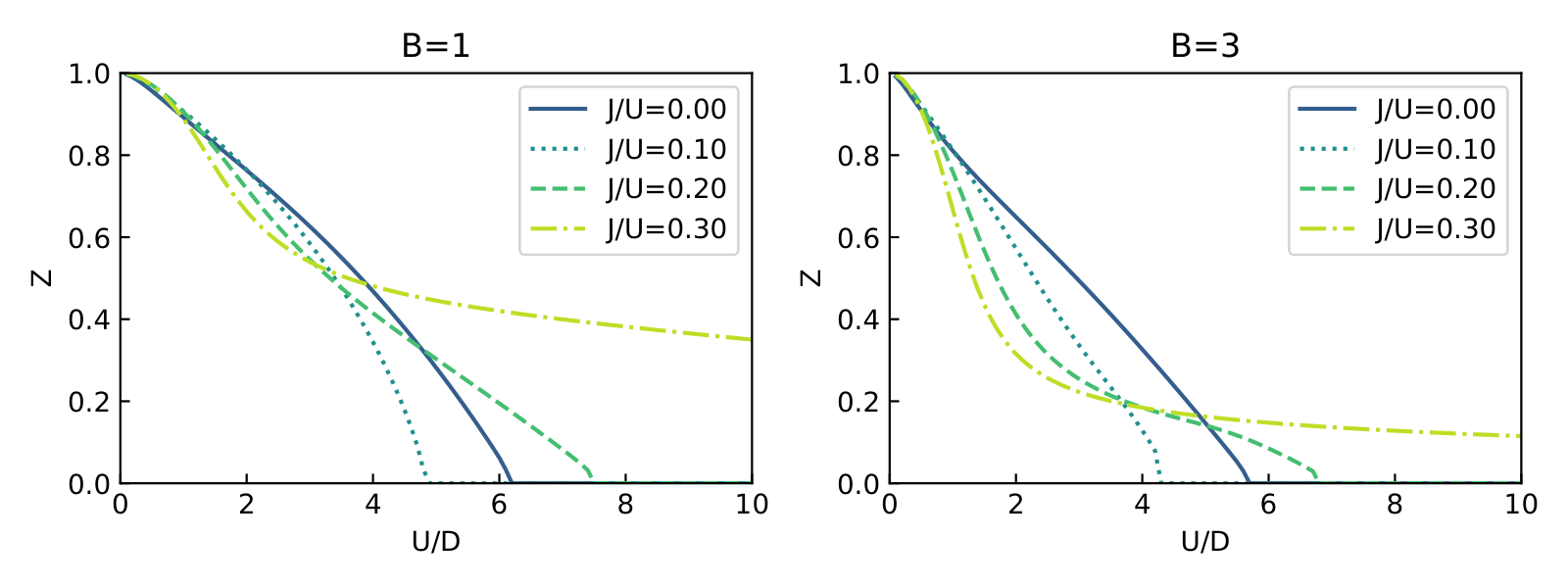
This example addresses the three-orbital Hubbard-Kanamori model on the Bethe lattice at fixed filling \(n = n_{orb} - 1\) (two electrons in three orbitals), and maps the quasiparticle weight \(Z\) as a function of \(U\) for several values of the Hund’s coupling \(J/U\). It is run both at \(B = 1\), i.e. the standard Gutzwiller approximation, and at \(B = 3\), so that the effect of the ghost levels on Hund’s physics can be read off directly.
Setup
Three orbitals with two spins give nimp = 6, and the embedding problem has
ntot = nimp * (B + 1) levels — 12 at \(B = 1\), 24 at \(B = 3\).
The interaction tensor is built by the helper
U_matrix_kanamori():
import numpy as np
from gem.fragment import Fragment
from gem.lattice import Lattice
from gem.solvers.simple_ed import SimpleED
from gem.utilities import U_matrix_kanamori

n_orb, B = 3, 3          # B is 1 or 3 in this example
nimp  = 2 * n_orb
nbath = nimp * B
ntot  = nimp + nbath

U_list, JoverU_list = np.linspace(0.1, 10.0, 100), np.array([0.00, 0.10, 0.20, 0.30])
T, n_target = 0, n_orb - 1

itmax, tol, mix, ntol, Tsmearing = 200, 1e-4, 0.2, 1e-4, 1e-3
The lattice is again the semicircular DOS of half-bandwidth 1, now with all
nimp spin-orbitals degenerate:
e_list = np.linspace(-1, 1, 1001)
wks = np.sqrt(1 - e_list**2)
wks /= np.sum(wks)
eks = e_list[:, None, None] * np.eye(nimp, dtype=np.complex128)
lattice = Lattice(eks, wk_list=wks)
Since the calculation runs at \(T = 0\), the solver can be restricted to the half-filled:
edsolver = SimpleED(ntot, use_Ntot=True, use_Sz=True,
                    N_sector=ntot//2, Sz_sector=0, dtype=np.float64)
Self-consistency loop
The scan is a double loop: for each \(J/U\), \(U\) is increased monotonically and the converged \(\Lambda\) and \(R\) (as well as \(\mu\)) are carried over as the starting guess for the next \(U\). This warm start is what keeps the solution on the same physical branch across the whole sweep, including through the strongly correlated region where several stationary points coexist:
for iJ, JoverU in enumerate(JoverU_list):
    Lambda0, R0, mu = None, None, 0
    for iU, U in enumerate(U_list):
        J = JoverU * U
        eloc = np.zeros((nimp, nimp))
        Utensor = U_matrix_kanamori(n_orb, U, J)

        fragment = Fragment(nimp, nbath, eloc, Utensor, edsolver,
                            Lambda=Lambda0, R=R0, verbose=0)
Note that eloc is left at zero: the level position is set entirely by the
chemical potential, which is refitted inside the loop whenever the impurity
filling drifts away from n_target by more than ntol:
for it in range(itmax):
    lattice.solve_qp([fragment], T=T, Tsmearing=Tsmearing)
    fragment.update_hybridization(T=T, use_Sz=True)
    fragment.solve_impurity(mu, T=T)

    if abs(fragment.nfill.real - n_target) > ntol:
        mu = lattice.fit_mu(n_target, [fragment], T=T, mu_old=mu,
                            mode='imp', ntol=1e-5)
        fragment.solve_impurity(mu, T=T)

    Lambda_old = fragment.Lambda.copy(); R_old = fragment.R.copy()
    fragment.update_self_energy(T=T, use_Sz=True)
    fragment.impose_orbital_symmetry()
    fragment.impose_spin_SU2_symmetry()

    fragment.Lambda = (1 - mix) * fragment.Lambda + mix * Lambda_old
    fragment.R      = (1 - mix) * fragment.R + mix * R_old
fit_mu is called with mode='imp', i.e. the target is the impurity
filling, and the impurity is re-solved immediately afterwards, since the
embedding problem depends on \(\mu\). The two symmetrisation calls,
impose_orbital_symmetry() and
impose_spin_SU2_symmetry(), project the updated
parameters back onto the paramagnetic, orbitally degenerate solution — without
them the sweep drifts into a spontaneously symmetry-broken sector at large
\(U\). Convergence is tested on the same gauge-invariant combination of
\(\Lambda\) eigenvalues and \(|R|\) used in E1,
here restricted to one spin-orbital per block.
Finally the quasiparticle weight and the filling are stored on the \((J/U, U)\) grid:
Z = fragment.compute_Z()
Zgrid[iJ, iU] = Z.real[0, 0]; ngrid[iJ, iU] = fragment.nfill.real
Lambda0 = fragment.Lambda.copy(); R0 = fragment.R.copy()
The grids are written into the B<B>/ subdirectory, one file each for
U_list, JoverU_list, Zgrid and ngrid.
Results
Results are plotted in the following figure for B=1 (left) and B=3 (right). The effect of the ghost levels is to show a much stronger suppression of the quasiparticle weight at large \(U\) when the Janus regime is entered.