Two-orbital Anderson impurity model

Here we illustrate calculations for multi-orbital models on the example of the two-orbital Anderson impurity model with inter-orbital charge and exchange (Hund’s) coupling with the Hamiltonian

\[ \begin{align}\begin{aligned}H_\mathrm{imp} = \sum_{i} \epsilon_i n_i + \sum_i U_i n_{i,\uparrow} n_{i,\downarrow} + U_{12} n_1 n_2 + J_{12} \mathbf{S}_1 \cdot \mathbf{S}_2\\where :math:\mathbf{S}_i are the spin operators:\\.. math::\\ \mathbf{S}_i = \frac{1}{2} d_{i\alpha}^\dagger \boldsymbol{\sigma}_{\alpha\beta} d_{i\beta}\end{aligned}\end{align} \]

Let us solve this problem with the NRG solver. Here is the python script:

from nrgljubljana_interface import Solver, Flat
from h5 import *
import math

# Parameters
D = 1.0 # bandwidth
U = 1.0
Gamma = 0.1
e_f = -0.4
U12 = 1.0
J12 = 0.0
T = 1e-3

# Set up the Solver
S = Solver(model = "2orb-UJ", symtype = "QS", mesh_max = 2.00676, mesh_min = 1e-5, mesh_ratio = 1.01)

# Solve Parameters
sp = { "T": T, "Lambda": 4.0, "Nz": 4, "Tmin": 1e-5, "keep": 4000, "keepenergy": 10.0, "bandrescale": 1.0 }

# Model Parameters
mp = { "U1": U, "U2": U, "eps1": e_f, "eps2": e_f, "U12": U12, "J12": J12 }
sp["model_parameters"] = mp

# Initialize hybridization function
S.Delta_w['imp'] << Gamma * (2.0/math.pi) * Flat(D)

# Solve the impurity model
S.solve(**sp)

# Store the Result
with HDFArchive("2orb-UJ_solution.h5", 'w') as arch:
    arch["A_w"] = S.A_w
    arch["G_w"] = S.G_w
    arch["F_w"] = S.F_w
    arch["Sigma_w"] = S.Sigma_w
    arch["expv"] = S.expv

print("<n>=", S.expv["n_d1"])
print("<n^2>=", S.expv["n_d1^2"])
print("<SS>=", S.expv["S_d1S_d2"])
print("<nn>=", S.expv["n_d1n_d2"])

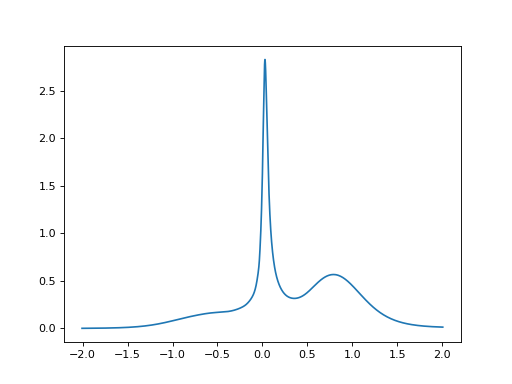
Running this script takes quite a bit of time and generates an HDF5 archive file called 2orb-UJ_solution.h5. This file contains the impurity spectral function, Green’s function, auxiliary Green’s function, self-energy, and some expectation values of local variables. Let us plot the spectral function:

import numpy as np
import matplotlib as mpl
import matplotlib.pyplot as plt
import math

from triqs.gf import *
from h5 import *
def A_to_nparrays(A):
    lx = np.array(list(A.mesh.values()))
    ly = np.array(A.data[:,0,0].real)
    return lx, ly

with HDFArchive('2orb-UJ_solution.h5','r') as ar:
    # Expectation values
    print("<n>=",ar['expv']['n_d1'])
    print("<n^2>=",ar['expv']['n_d1^2'])

    # Spectral function
    A_w = ar['A_w']['imp']
    lx, ly = A_to_nparrays(A_w)
    plt.plot(lx, ly)
    plt.show()