Tools for analysis

This section explains how to use some tools of the package in order to analyse the data. There are certain tools here which are not available for some DFT code interfaces. Please refer to the DFT package interface converter documentation (see Supported interfaces) on how to interface the required DFT outputs into the HDF5 files needed for the tools discussed here. This section will assume that the user has converted the required DFT data.

The following routines require a self energy on the real frequency axis if the user specifies the inputs with_Sigma and with_dc:

density_of_states for the momentum-integrated spectral function including self energy effects and

spaghettis for the momentum-resolved spectral function (i.e. ARPES)

spectral_contours for the k-resolved spectral function on a specific k-mesh (i.e., spectral function on a two dimensional k-mesh)

Note

This package does NOT provide an explicit method to do an analytic continuation of self energies and Green functions from Matsubara frequencies to the real-frequency axis, but a list of options available within the TRIQS framework is given here. Keep in mind that all these methods have to be used very carefully!

Otherwise, without these options, the spectral functions from the inputs of the interfaced DFT code will be used.

The other routines presented here use the Matsubara self-energy.

Initialisation

All tools described below are collected in an extension of the SumkDFT class and are loaded by importing the module SumkDFTTools:

from triqs_dft_tools.sumk_dft_tools import *

The initialisation of the class is equivalent to that of the SumkDFT class:

SK = SumkDFTTools(hdf_file = filename + '.h5')

Note that all routines available in SumkDFT are also available here.

If required, we have to load and initialise the real-frequency self energy. Most conveniently, you have your self energy already stored as a real-frequency BlockGf object in a hdf5 file:

with HDFArchive('case.h5', 'r') as ar:
      SigmaReFreq = ar['dmft_output']['Sigma_w']

You may also have your self energy stored in text files. For this case the TRIQS library offers the function read_gf_from_txt(), which is able to load the data from text files of one Green function block into a real-frequency ReFreqGf object. Loading each block separately and building up a :class:´BlockGf <triqs.gf.BlockGf>´ is done with:

from triqs.gf.tools import *
# get block names
n_list = [n for n,nl in SK.gf_struct_solver[0].iteritems()]
# load sigma for each block - in this example sigma is composed of 1x1 blocks
g_blocks = [read_gf_from_txt(block_txtfiles=[['Sigma_'+name+'.dat']], block_name=n) for n in n_list]
# put the data into a BlockGf object
SigmaReFreq = BlockGf(name_list=n_list, block_list=g_blocks, make_copies=False)

where:

block_txtfiles is a rank 2 square np.array(str) or list[list[str]] holding the file names of one block and

block_name is the name of the block.

It is important that each data file has to contain three columns: the real-frequency mesh, the real part and the imaginary part of the self energy - exactly in this order! The mesh should be the same for all files read in and non-uniform meshes are not supported.

Finally, we set the self energy into the SK object:

SK.set_Sigma([SigmaReFreq])

and additionally set the chemical potential and the double counting correction from the DMFT calculation:

chemical_potential, dc_imp, dc_energ = SK.load(['chemical_potential','dc_imp','dc_energ'])
SK.set_mu(chemical_potential)
SK.set_dc(dc_imp,dc_energ)

Density of states

For plotting the density of states, you type:

SK.density_of_states(mu, broadening, mesh, with_Sigma, with_dc, proj_type, dosocc, save_to_file)

where a description of all of the inputs are given in density_of_states:

SumkDFTTools.density_of_states(mu=None, broadening=None, mesh=None, with_Sigma=True, with_dc=True, proj_type=None, dosocc=False, save_to_file=True)[source]

Calculates the density of states and the projected density of states. The basis of the projected density of states is specified by proj_type.

The output files (if save_to_file = True) have two (three in the orbital-resolved case) columns representing the frequency and real part of the DOS (and imaginary part of the DOS) in that order.

The output files are as follows:

DOS_(spn).dat, the total DOS.
DOS_(proj_type)_(spn)_proj(i).dat, the DOS projected to an orbital with index i which refers to the index given in SK.shells (or SK.corr_shells for proj_type = “wann”).
DOS_(proj_type)_(sp)_proj(i)_(m)_(n).dat, As above, but printed as orbitally-resolved matrix in indices “m” and “n”. For example, for “d” orbitals, it gives the DOS separately for each orbital (e.g., d_(xy), d_(x^2-y^2), and so on).

Parameters:

mu : double, optional

Chemical potential, overrides the one stored in the hdf5 archive. By default, this is automatically set to the chemical potential within the SK object.

broadening : double, optional

Lorentzian broadening of the spectra to avoid any numerical artifacts. If not given, standard value of lattice_gf (0.001 eV) is used.

mesh : real frequency MeshType, optional

Omega mesh for the real-frequency Green’s function. Given as parameter to lattice_gf.

with_Sigma : boolean, optional

If True, the self energy is used for the calculation. If false, the DOS is calculated without self energy. Both with_Sigma and with_dc equal to True is needed for DFT+DMFT A(w) calculated. Both with_Sigma and with_dc equal to false is needed for DFT A(w) calculated.

with_dc : boolean, optional

If True the double counting correction is used.

proj_type : string, optional

The type of projection used for the orbital-projected DOS. These projected spectral functions will be determined alongside the total spectral function. By default, no projected DOS type will be calculated (the corresponding projected arrays will be empty). The following options are:

‘None’ - Only total DOS calculated ‘wann’ - Wannier DOS calculated from the Wannier projectors ‘vasp’ - Vasp orbital-projected DOS only from Vasp inputs ‘wien2k’ - Wien2k orbital-projected DOS from the wien2k theta projectors

dosocc : boolean, optional

If True, the occupied DOS, DOSproj and DOSproj_orb will be returned. The prerequisite of this option is to have calculated the band-resolved density matrices generated by the occupations() routine.

save_to_file : boolean, optional

If True, text files with the calculated data will be created.

Returns:

DOS : Dict of numpy arrays

Contains the full density of states with the form of DOS[spn][n_om] where “spn” speficies the spin type of the calculation (“up”, “down”, or combined “ud” which relates to calculations with spin-orbit coupling) and “n_om” is the number of real frequencies as specified by the real frequency MeshType used in the calculation. This array gives the total density of states.

DOSproj : Dict of numpy arrays

DOS projected to atom (shell) with the form of DOSproj[n_shells][spn][n_om] where “n_shells” is the total number of correlated or uncorrelated shells (depending on the input “proj_type”). This array gives the trace of the orbital-projected density of states. Empty if proj_type = None

DOSproj_orb : Dict of numpy arrays

Orbital-projected DOS projected to atom (shell) and resolved into orbital contributions with the form of DOSproj_orb[n_shells][spn][n_om,dim,dim] where “dim” specifies the orbital dimension of the correlated/uncorrelated shell (depending on the input “proj_type”). Empty if proj_type = None

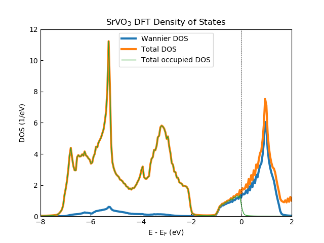
The figure above shows the DFT SrVO₃ density of states generated from 2925 k-points in the irreducible Brillouin zone with the V t_2g Wannier projectors generated within a correlated energy window of [-13.6, 13.6] eV. The broadening input has been set to the temperature (i.e., 1/Beta). The total, V t_2g Wannier and occupied total density of states generated from the SK.density_of_states() routine are shown. Note that the noise in the density of states comes from the number of k-points used. This can be removed upon by either using more k-points or using a larger broadening value.

Band resolved density matrices

Calculates the band resolved density matrices (occupations) from the Matsubara frequency self-energy. This is done by calling the following:

SK.occupations(mu, with_Sigma, with_dc, save_occ):

This is required to generate the occupied DOS in SK.density_of_states() when dosocc is set to True. The save_occ optional input (True by default) saves these density matrices to the HDF5 file within the misc_data subgroup. The other variables are the same as defined above. See occupations

Momentum resolved spectral function (with real-frequency self energy)

Another quantity of interest is the calculated momentum-resolved spectral function A(k, \(\omega\)) or (correlated) band structure which can directly be compared to ARPES experiments. First we have generate the required files from the DFT code of choice and interface them with DFT_Tools, see the guides of the DFT converters (Supported interfaces) on how to do this.

This spectral function is calculated by typing:

SK.spaghettis(mu, broadening, mesh, plot_shift, plot_range, shell_list, with_Sigma, with_dc, proj_type, save_to_file)

SumkDFTTools.spaghettis(mu=None, broadening=None, mesh=None, plot_shift=0.0, plot_range=None, shell_list=None, with_Sigma=True, with_dc=True, proj_type=None, save_to_file=True)[source]

Calculates the k-resolved spectral function A(k,w) (band structure)

The output files have three columns representing the k-point index, frequency and A(k,w) (in this order).

The output files are as follows:

Akw_(sp).dat, the total A(k,w).
Akw_(proj_type)_(spn)_proj(i).dat, the A(k,w) projected to shell with index (i).
Akw_(proj_type)_(spn)_proj(i)_(m)_(n).dat, as above, but for each (m) and (n) orbital contribution.

Parameters:

mu : double, optional

Chemical potential, overrides the one stored in the hdf5 archive. By default, this is automatically set to the chemical potential within the SK object.

broadening : double, optional

Lorentzian broadening of the spectra to avoid any numerical artifacts. If not given, standard value of lattice_gf (0.001 eV) is used.

mesh : real frequency MeshType, optional

Omega mesh for the real-frequency Green’s function. Given as parameter to lattice_gf.

plot_shift : double, optional

Offset [=(ik-1)*plot_shift, where ik is the index of the k-point] for each A(k,w) for stacked plotting of spectra.

plot_range : list of double, optional

Sets the energy window for plotting to (plot_range[0],plot_range[1]). If not provided, the min and max values of the energy mesh is used.

shell_list : list of integers, optional

Contains the indices of the shells of which the projected spectral function is calculated for. If shell_list = None and proj_type is not None, then the projected spectral function is calculated for all shells. Note for experts: The spectra from Wien2k inputs are not rotated to the local coordinate system used in Wien2k.

with_Sigma : boolean, optional

If True, the self energy is used for the calculation. If false, the DOS is calculated without self energy. Both with_Sigma and with_dc equal to True is needed for DFT+DMFT A(k,w) calculated. Both with_Sigma and with_dc equal to false is needed for DFT A(k,w) calculated.

with_dc : boolean, optional

If True the double counting correction is used.

proj_type : string, optional

The type of projection used for the orbital-projected DOS. These projected spectral functions will be determined alongside the total spectral function. By default, no projected DOS type will be calculated (the corresponding projected arrays will be empty). The following options are:

‘None’ - Only total DOS calculated ‘wann’ - Wannier DOS calculated from the Wannier projectors ‘wien2k’ - Wien2k orbital-projected DOS from the wien2k theta projectors

save_to_file : boolean, optional

If True, text files with the calculated data will be created.

Returns:

Akw : Dict of numpy arrays

(Correlated) k-resolved spectral function. This dictionary has the form of Akw[spn][n_k, n_om] where spn, n_k and n_om are the spin, number of k-points, and number of frequencies used in the calculation.

pAkw : Dict of numpy arrays

(Correlated) k-resolved spectral function projected to atoms (i.e., the Trace of the orbital-projected A(k,w)). This dictionary has the form of pAkw[n_shells][spn][n_k, n_om] where n_shells is the total number of correlated or uncorrelated shells. Empty if proj_type = None

pAkw_orb : Dict of numpy arrays

(Correlated) k-resolved spectral function projected to atoms and resolved into orbital contributions. This dictionary has the form of pAkw[n_shells][spn][n_k, n_om,dim,dim] where dim specifies the orbital dimension of the correlated/uncorrelated shell. Empty if proj_type = None

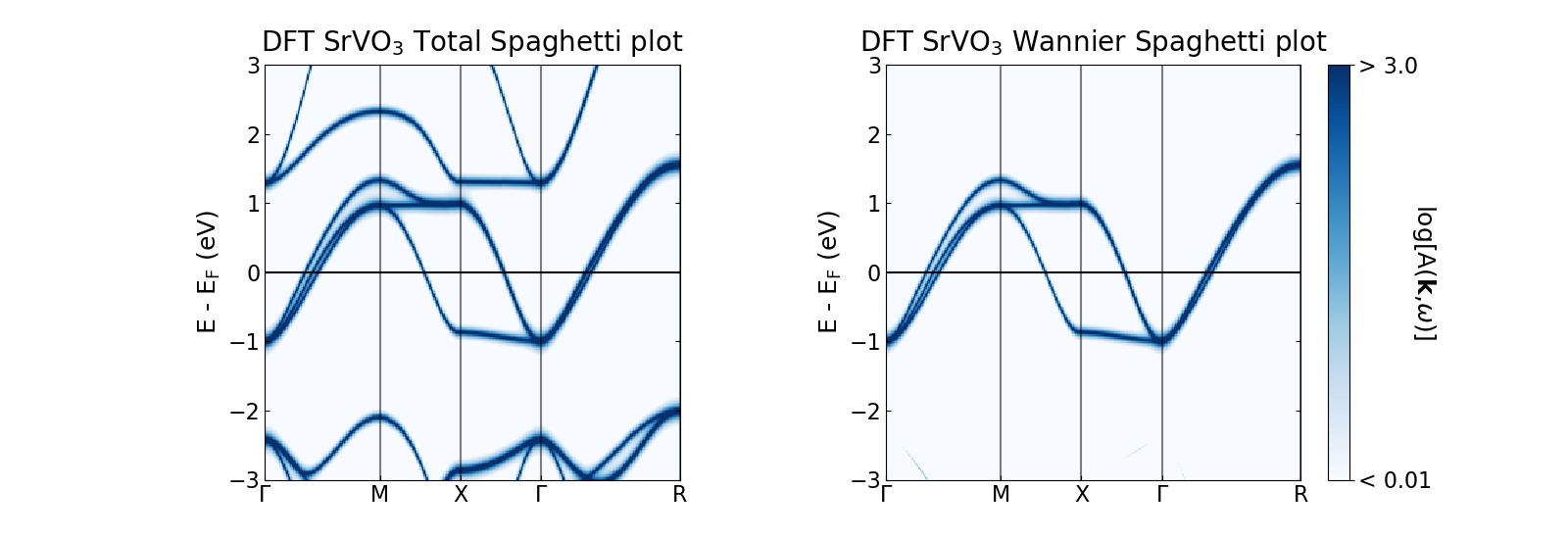
../_images/DFT_Tools_SVO_DFT_spaghettis.png

The figure above shows the DFT SrVO₃ spaghetti plot (generated using V t_2g Wannier projectors generated within a correlated energy window of [-13.6, 13.6] eV). As before, the broadening input has been set to the temperature (i.e., 1/Beta). The left panel shows the total A(k, \(\omega\)) whereas the right gives the Wannier A(k, \(\omega\)), both generated from this SK.spaghettis().

Energy contours of the k-resolved Spectral function

Currently, this has only been implemented for Elk DFT inputs only.

This routine calculates the k-resolved spectral function evaluated at the Fermi level or several energy contours on the k-mesh defined in the converter stage:

SK.spectral_contours(mu, broadening, mesh, plot_range, FS, with_Sigma, with_dc, proj_type, save_to_file)

SumkDFTTools.spectral_contours(mu=None, broadening=None, mesh=None, plot_range=None, FS=True, with_Sigma=True, with_dc=True, proj_type=None, save_to_file=True)[source]

Calculates the correlated spectral function at the Fermi level (relating to the Fermi surface) or at specific frequencies.

The output files have three columns representing the k-point index, frequency and A(k,w) in that order. The output files are as follows:

Akw_(sp).dat, the total A(k,w)
Akw_(proj_type)_(spn)_proj(i).dat, the A(k,w) projected to shell with index (i).
Akw_(proj_type)_(spn)_proj(i)_(m)_(n).dat, as above, but for each (m) and (n) orbital contribution.

The files are prepended with either of the following: For FS set to True the output files name include _FS_ and these files contain four columns which are the cartesian reciprocal coordinates (kx, ky, kz) and Akw. For FS set to False the output files name include _omega_(iom) (with iom being the frequency mesh index). These files also contain four columns as described above along with a comment at the top of the file which gives the frequency value at which the spectral function was evaluated.

Parameters:

mu : double, optional

Chemical potential, overrides the one stored in the hdf5 archive. By default, this is automatically set to the chemical potential within the SK object.

broadening : double, optional

Lorentzian broadening of the spectra to avoid any numerical artifacts. If not given, standard value of lattice_gf (0.001 eV) is used.

mesh : real frequency MeshType, optional

Omega mesh for the real-frequency Green’s function. Given as parameter to lattice_gf.

plot_shift : double, optional

Offset [=(ik-1)*plot_shift, where ik is the index of the k-point] for each A(k,w) for stacked plotting of spectra.

plot_range : list of double, optional

Sets the energy window for plotting to (plot_range[0],plot_range[1]). If not provided, the min and max values of the energy mesh is used.

FS : boolean

Flag for calculating the spectral function at the Fermi level (omega ~ 0) If False, the spectral function will be generated for each frequency within plot_range.

with_Sigma : boolean, optional

If True, the self energy is used for the calculation. If false, the DOS is calculated without self energy. Both with_Sigma and with_dc equal to True is needed for DFT+DMFT A(k,w) calculated. Both with_Sigma and with_dc equal to false is needed for DFT A(k,w) calculated.

with_dc : boolean, optional

If True the double counting correction is used.

proj_type : string, optional

The type of projection used for the orbital-projected DOS. These projected spectral functions will be determined alongside the total spectral function. By default, no projected DOS type will be calculated (the corresponding projected arrays will be empty). The following options are:

None Only total DOS calculated

wann Wannier DOS calculated from the Wannier projectors

save_to_file : boolean, optional

If True, text files with the calculated data will be created.

Returns:

Akw : Dict of numpy arrays

(Correlated) k-resolved spectral function. This dictionary has the form of Akw[spn][n_k, n_om] where spn, n_k and n_om are the spin, number of k-points, and number of frequencies used in the calculation.

pAkw : Dict of numpy arrays

(Correlated) k-resolved spectral function projected to atoms (i.e., the Trace of the orbital-projected A(k,w)). This dictionary has the form of pAkw[n_shells][spn][n_k, n_om] where n_shells is the total number of correlated or uncorrelated shells. Empty if proj_type = None

pAkw_orb : Dict of numpy arrays

(Correlated) k-resolved spectral function projected to atoms and resolved into orbital contributions. This dictionary has the form of pAkw[n_shells][spn][n_k, n_om,dim,dim] where dim specifies the orbital dimension of the correlated/uncorrelated shell. Empty if proj_type = None

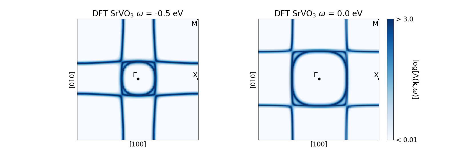
../_images/DFT_Tools_SVO_DFT_energy_contours.png

The figure above shows the DFT SrVO₃ energy contour plots (again, generated using V t_2g Wannier projectors generated within a correlated energy window of [-13.6, 13,6] eV and broadening of 1/Beta). Both panels have been generated on a k-mesh within the first Brillouin zone on the k_z= 0.0 plane centered at the \(\Gamma\) point. Here, each panel generated using the outputs from this SK.spectral_contours_plot() routine shows the A(k, \(\omega\)) evaluated at \(\omega\) = -0.5 eV (left) and the Fermi level, \(\omega\) = 0.0 eV, (right).

Partial charges

Currently, this has only been implemented for Wien2k DFT inputs only.

Since we can calculate the partial charges directly from the Matsubara Green functions, we also do not need a real-frequency self energy for this purpose. The calculation is done by:

SK.set_Sigma(SigmaImFreq)
dm = SK.partial_charges(beta=40.0, with_Sigma=True, with_dc=True)

which calculates the partial charges using the self energy, double counting, and chemical potential as set in the SK object. On return, dm is a list, where the list items correspond to the density matrices of all shells defined in the list SK.shells. This list is constructed by the Wien2k converter routines and stored automatically in the hdf5 archive. For the structure of dm, see also partial charges.