Transport calculations
Formalism
The conductivity, the Seebeck coefficient and the electronic contribution to the thermal conductivity in direction \(\alpha\beta\) are defined as [1] [2]:
in which the kinetic coefficients \(A_{n,\alpha\beta}\) are given by
Here \(N_{sp}\) is the spin factor and \(f(\omega)\) is the Fermi function. The transport distribution \(\Gamma_{\alpha\beta}\left(\omega_1,\omega_2\right)\) is defined as
where \(V\) is the unit cell volume. In multi-band systems the velocities \(v_{k}\) and the spectral function \(A(k,\omega)\) are matrices in the band indices \(i\) and \(j\). The frequency depended optical conductivity is given by
Prerequisites
First perform a standard DFT+DMFT calculation for your desired material and obtain the real-frequency self energy.
Note
If you use a CT-QMC impurity solver you need to perform an analytic continuation of self energies and Green functions from Matsubara frequencies to the real-frequency axis! This packages does NOT provide methods to do this, but a list of options available within the TRIQS framework is given here. Keep in mind that all these methods have to be used very carefully. Especially for optics calculations it is crucial to perform the analytic continuation in such a way that the real-frequency self energy is accurate around the Fermi energy as low-energy features strongly influence the final results.
Below will describe the prerequisites from the different DFT codes.
Prequisites from Wien2k
- Besides the self energy the Wien2k files read by the transport converter (
convert_transport_input) are: .struct: The lattice constants specified in the struct file are used to calculate the unit cell volume..outputs: In this file the k-point symmetries are given..oubwin: Contains the indices of the bands within the projected subspace (written by dmftproj) for each k-point..pmat: This file is the output of the Wien2k optics package and contains the velocity (momentum) matrix elements between all bands in the desired energy window for each k-point. How to use the optics package is described below..h5: The hdf5 archive has to be present and should contain the dft_input subgroup. Otherwiseconvert_dft_inputneeds to be called beforeconvert_transport_input.
These Wien2k files are read and the relevant information is stored in the hdf5 archive by using the following:
from triqs_dft_tools.converters import Wien2kConverter
from triqs_dft_tools.sumk_dft_tools import *

Converter = Wien2kConverter(filename='case', repacking=True)
Converter.convert_transport_input()

SK = SumkDFTTools(hdf_file='case.h5', use_dft_blocks=True)
The converter convert_transport_input
reads the required data of the Wien2k output and stores it in the dft_transp_input subgroup of your hdf file.
Wien2k optics package
- The basics steps to calculate the matrix elements of the momentum operator with the Wien2k optics package are:
Perform a standard Wien2k calculation for your material.
Run x kgen to generate a dense k-mesh.
Run x lapw1.
For metals change TETRA to 101.0 in
case.in2.Run x lapw2 -fermi.
Run x optic.
Additionally the input file case.inop is required. A detail description on how to setup this file can be found in the Wien2k user guide [3] on page 166.
The optics energy window should be chosen according to the window used for dmftproj. Note that the current version of the transport code uses only the smaller
of those two windows. However, keep in mind that the optics energy window has to be specified in absolute values and NOT relative to the Fermi energy!
You can read off the Fermi energy from the case.scf2 file. Please do not set the optional parameter NBvalMAX in case.inop.
Furthermore it is necessary to set line 6 to “ON” and put a “1” in the following line to enable the printing of the matrix elements to case.pmat.
Prequisites from Elk
- The Elk transport converter (
convert_transport_input) reads in the following files: LATTICE.OUT: Real and reciprocal lattice structure and cell volumes.
SYMCRYS.OUT: Crystal symmetries.
PMAT.OUT: Fortran binary containing the velocity matrix elements.
.h5: The hdf5 archive has to be present and should contain the dft_input subgroup. Otherwiseconvert_dft_inputneeds to be called beforeconvert_transport_input. It is recommended to callconvert_dft_inputbeforeconvert_transport_input.
Except for PMAT.OUT, the other files are standard outputs from Elk’s groundstate calculation and are used in convert_dft_input. The PMAT.OUT file on the otherhand is generated by Elk by running task 120, see [4]. Note that unlike in the Wien2k transport converter, the Elk transport converter uses the correlated band window stored in the dft_misc_input (which originates from running convert_dft_input).
These Elk files are then read and the relevant information is stored in the hdf5 archive by using the following:
from triqs_dft_tools.converters import ElkConverter
from triqs_dft_tools.sumk_dft_tools import *

Converter = ElkConverter(filename='case', repacking=True)
Converter.convert_transport_input()

SK = SumkDFTTools(hdf_file='case.h5', use_dft_blocks=True)
The converter convert_transport_input
reads the required data of the Elk output and stores it in the dft_transp_input subgroup of your hdf file.
Using the transport code
Once we have converted the transport data from the DFT codes (see above), we also need to read and set the self energy, the chemical potential and the double counting:
with HDFArchive('case.h5', 'r') as ar:
    SK.set_Sigma([ar['dmft_output']['Sigma_w']])
    chemical_potential,dc_imp,dc_energ = SK.load(['chemical_potential','dc_imp','dc_energ'])
    SK.set_mu(chemical_potential)
    SK.set_dc(dc_imp,dc_energ)
As next step we can calculate the transport distribution \(\Gamma_{\alpha\beta}(\omega)\):
SK.transport_distribution(directions=['xx'], Om_mesh=[0.0, 0.1], energy_window=[-0.3,0.3],
                                             with_Sigma=True, broadening=0.0, beta=40)
Here the transport distribution is calculated in \(xx\) direction for the frequencies \(\Omega=0.0\) and \(0.1\).
To use the previously obtained self energy we set with_Sigma to True and the broadening to \(0.0\).
As we also want to calculate the Seebeck coefficient and the thermal conductivity we have to include \(\Omega=0.0\) in the mesh.
Note that the current version of the code repines the \(\Omega\) values to the closest values on the self energy mesh.
For complete description of the input parameters see the transport_distribution reference.
The resulting transport distribution is not automatically saved, but this can be easily achieved with:
SK.save(['Gamma_w','Om_mesh','omega','directions'])
You can retrieve it from the archive by:
SK.Gamma_w, SK.Om_mesh, SK.omega, SK.directions = SK.load(['Gamma_w','Om_mesh','omega','directions'])
Finally the optical conductivity \(\sigma(\Omega)\), the Seebeck coefficient \(S\) and the thermal conductivity \(\kappa^{\text{el}}\) can be obtained with:
SK.conductivity_and_seebeck(beta=40)
SK.save(['seebeck','optic_cond','kappa'])
It is strongly advised to check convergence in the number of k-points!
Example
Here we present an example calculation of the DFT optical conductivity of SrVO3 comparing the results from the Elk and Wien2k inputs. The DFT codes used 4495 k-points in the irreducible Brillouin zone with Wannier projectors generated within a correlated energy window of [-8, 7.5] eV. We assume that the required DFT files have been read and saved by the TRIQS interface routines as discussed previously. Below is an example script to generate the conductivities:
from sumk_dft_tools import *
import numpy

SK = SumkDFTTools(hdf_file=filename+'.h5', use_dft_blocks=True)

#Generate numpy mesh for omega values
om_mesh = list(numpy.linspace(0.0,5.0,51))

#Generate and save the transport distribution
SK.transport_distribution(directions=['xx'], Om_mesh=om_mesh, energy_window=[-8.0, 7.5], with_Sigma=False, broadening=-0.05, beta=40, n_om=1000)
SK.save(['Gamma_w','Om_mesh','omega','directions'])

#Generate and save conductivities
SK.conductivity_and_seebeck(beta=40)
SK.save(['seebeck','optic_cond','kappa'])
The optic_cond variable can be loaded by using SK.load() and then plotted to generate the following figure.
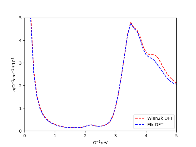
Note that the differences between the conductivities arise from the differences in the velocities generated in the DFT codes. The DMFT optical conductivity can easily be calculated by adjusting the above example script by setting with_Sigma to True. In this case however, the SK object will need the DMFT self-energy on the real frequency axis.