DFT+DMFT tutorial: Ce with Hubbard-I approximation
In this tutorial we will perform DFT+DMFT Wien2k calculations from scratch, including all steps described in the previous sections. As example, we take the high-temperature \(\gamma\)-phase of Ce employing the Hubbard-I approximation for its localized 4f shell.
Wien2k setup
First we create the Wien2k Ce-gamma.struct file as described in the
Wien2k manual
for the \(\gamma\)-Ce fcc structure with lattice parameter of 9.75 a.u.
Title
F   LATTICE,NONEQUIV.ATOMS:  1225_Fm-3m
MODE OF CALC=RELA unit=bohr
  9.750000  9.750000  9.750000 90.000000 90.000000 90.000000
ATOM   1: X=0.00000000 Y=0.00000000 Z=0.00000000
          MULT= 1          ISPLIT= 2
Ce         NPT=  781  R0=0.00001000 RMT=    2.5000   Z: 58.0
LOCAL ROT MATRIX:    1.0000000 0.0000000 0.0000000
                     0.0000000 1.0000000 0.0000000
                     0.0000000 0.0000000 1.0000000
   0      NUMBER OF SYMMETRY OPERATIONS
We initalize non-magnetic Wien2k calculations using the init script as described in the same manual. For this example we specify 3000 \(\mathbf{k}\)-points in the full Brillouin zone and LDA exchange-correlation potential (vxc=5), other parameters are defaults. The Ce 4f electrons are treated as valence states. Hence, the initialization script is executed as follows
init -b -vxc 5 -numk 3000
and then LDA calculations of non-magnetic \(\gamma\)-Ce are performed by launching the Wien2k run script. These self-consistent LDA calculations will typically take a couple of minutes.
Wannier orbitals: dmftproj
Then we create the Ce-gamma.indmftpr file specifying parameters for construction
of Wannier orbitals representing 4f states:
1                ! Nsort
1                ! Mult(Nsort)
3                ! lmax
complex
1 1 1 2          ! l included for each sort
0 0 0 0          ! l included for each sort
0
-.40 0.40         ! Energy window relative to E_f
As we learned in the section Supported interfaces, the first three lines give the number of inequivalent sites, their multiplicity (to be in accordance with the struct file) and the maximum orbital quantum number \(l_{max}\). The following four lines describe the treatment of Ce spdf orbitals by the dmftproj program:
complex
1 1 1 2          ! l included for each sort
0 0 0 0          ! l included for each sort
0
where complex is the choice for the angular basis to be used (spherical complex harmonics), in the next line we specify, for each orbital quantum number, whether it is treated as correlated (‘2’) and, hence, the corresponding Wannier orbitals will be generated, or uncorrelated (‘1’). In the latter case the dmftproj program will generate projectors to be used in calculations of corresponding partial densities of states (see below). In the present case we choose the fourth (i. e. f) orbitals as correlated. The next line specify the number of irreducible representations into which a given correlated shell should be split (or ‘0’ if no splitting is desired, as in the present case). The fourth line specifies whether the spin-orbit interaction should be switched on (‘1’) or off (‘0’, as in the present case).
Finally, the last line of the file
-.40 0.40 ! Energy window relative to E_f
specifies the energy window for Wannier functions’ construction. For a more complete description of dmftproj options see its manual.
To prepare input data for dmftproj we execute lapw2 with the -almd option
x lapw2 -almd
Then dmftproj is executed in its default mode (i.e. without spin-polarization or spin-orbit included)
dmftproj
This program produces the following files:
Ce-gamma.ctqmcoutandCe-gamma.symqmccontaining projector operators and symmetry operations for orthonormalized Wannier orbitals, respectively.
Ce-gamma.parprojandCe-gamma.symparcontaining projector operators and symmetry operations for uncorrelated states, respectively. These files are needed for projected density-of-states or spectral-function calculations.
Ce-gamma.oubwinneeded for the charge density recalculation in the case of a fully self-consistent DFT+DMFT run (see below).
Now we have all necessary input from Wien2k for running DMFT calculations.
DMFT setup: Hubbard-I calculations in TRIQS
In order to run DFT+DMFT calculations within Hubbard-I we need the corresponding python script, Ce-gamma.py. It is generally similar to the script for the case of DMFT calculations with the CT-QMC solver (see Single-shot DFT+DMFT), however there are also some differences. First difference is that we import the Hubbard-I solver by:
from triqs.applications.impurity_solvers.hubbard_I.hubbard_solver import Solver
The Hubbard-I solver is very fast and we do not need to take into account the DFT block structure
or use any approximation for the U-matrix. We load and convert the dmftproj output
and initialize the SumkDFT class as described in Supported interfaces and
Single-shot DFT+DMFT and then set up the Hubbard-I solver
S = Solver(beta = beta, l = l)
where the solver is initialized with the value of beta, and the orbital quantum number l (equal to 3 in our case).
The Hubbard-I initialization Solver has also optional parameters one may use:
n_msb: the number of Matsubara frequencies used. The default is n_msb=1025.
use_spin_orbit: if set ‘True’ the solver is run with spin-orbit coupling included. To perform actual DFT+DMFT calculations with spin-orbit one should also run Wien2k and dmftproj in spin-polarized mode and with spin-orbit included. By default, use_spin_orbit=False.
Nmoments: the number of moments used to describe high-frequency tails of the Hubbard-I Green function and self energy. By default Nmoments = 5
The Solver.solve(U_int, J_hund) statement has two necessary parameters, the Hubbard U parameter U_int and Hund’s rule coupling J_hund. Notice that the solver constructs the full 4-index U-matrix by default, and the U_int parameter is in fact the Slater F0 integral. Other optional parameters are:
T: matrix that transforms the interaction matrix from complex spherical harmonics to a symmetry adapted basis. By default, the complex spherical harmonics basis is used and T=None.
verbosity: tunes output from the solver. If verbosity=0 only basic information is printed, if verbosity=1 the ground state atomic occupancy and its energy are printed, if verbosity=2 additional information is printed for all occupancies that were diagonalized. By default, verbosity=0.
Iteration_Number: the iteration number of the DMFT loop. Used only for printing. By default Iteration_Number=1
Test_Convergence: convergence criterion. Once the self energy is converged below Test_Convergence the Hubbard-I solver is not called anymore. By default Test_Convergence=0.0001.
We need also to introduce some changes in the DMFT loop with respect that used for CT-QMC calculations in Single-shot DFT+DMFT. The hybridization function is neglected in the Hubbard-I approximation, and only non-interacting level positions (\(\hat{\epsilon}=-\mu+\langle H^{ff} \rangle - \Sigma_{DC}\)) are required. Hence, instead of computing S.G0 as in Single-shot DFT+DMFT we set the level positions:
# set atomic levels:
eal = SK.eff_atomic_levels()[0]
S.set_atomic_levels( eal = eal )
The part after the solution of the impurity problem remains essentially the same: we mix the self energy and local Green function and then save them in the hdf5 file. Then the double counting is recalculated and the correlation energy is computed with the Migdal formula and stored in hdf5.
Finally, we compute the modified charge density and save it as well as correlation correction to the total energy in
Ce-gamma.qdmft file, which is then read by lapw2 in the case of self-consistent DFT+DMFT calculations.
You should try to run your script before setting up the fully charge self-consistent calculation (see this page).
Fully charge self-consistent DFT+DMFT calculation
Instead of doing only one-shot runs we perform in this tutorial a fully self-consistent DFT+DMFT calculations. We launch such a calculations with
run -qdmft 1
where -qdmft flag turns on DFT+DMFT calculations with Wien2k, and one computing core. We use here the default convergence criterion in Wien2k (convergence to 0.1 mRy in energy).
After calculations are done we may check the value of correlation (‘Hubbard’) energy correction to the total energy:
>grep HUBBARD Ce-gamma.scf|tail -n 1
HUBBARD ENERGY(included in SUM OF EIGENVALUES):           -0.012866
In the case of Ce, with the correlated shell occupancy close to 1 the Hubbard energy is close to 0, while the DC correction to energy is about J/4 in accordance with the fully-localized-limit formula, hence, giving the total correction \(\Delta E_{HUB}=E_{HUB}-E_{DC} \approx -J/4\), which is in our case is equal to -0.175 eV \(\approx\)-0.013 Ry.
The band (“kinetic”) energy with DMFT correction is
>grep DMFT Ce-gamma.scf |tail -n 1
KINETIC ENERGY with DMFT correction:                      -5.370632
One may also check the convergence in total energy:
>grep :ENE Ce-gamma.scf |tail -n 5
:ENE  : ********** TOTAL ENERGY IN Ry =       -17717.56318334
:ENE  : ********** TOTAL ENERGY IN Ry =       -17717.56342250
:ENE  : ********** TOTAL ENERGY IN Ry =       -17717.56271503
:ENE  : ********** TOTAL ENERGY IN Ry =       -17717.56285812
:ENE  : ********** TOTAL ENERGY IN Ry =       -17717.56287381
Post-processing and data analysis
Within Hubbard-I one may also easily obtain the angle-resolved spectral function (band structure) and integrated spectral function (density of states or DOS). In difference with the CT-QMC approach one does not need to do an analytic continuations to get the real-frequency self energy, as it can be calculated directly in the Hubbard-I solver.
The corresponding script Ce-gamma_DOS.py contains several new parameters
ommin=-4.0    # bottom of the energy range for DOS calculations
ommax=6.0     # top  of the energy range for DOS calculations
N_om=2001     # number of points on the real-energy axis mesh
broadening = 0.02 # broadening (the imaginary shift of the real-energy mesh)
Then one needs to load projectors needed for calculations of corresponding projected densities of states, as well as corresponding symmetries:
Converter.convert_parpoj_input()
To get access to analysing tools we initialize the
SumkDFTTools class
SK = SumkDFTTools(hdf_file=dft_filename+'.h5', use_dft_blocks=False)
After the solver initialization, we load the previously calculated chemical potential and double-counting correction. Having set up atomic levels we then compute the atomic Green function and self energy on the real axis:
S.set_atomic_levels(eal=eal)
S.GF_realomega(ommin=ommin, ommax=ommax, N_om=N_om, U_int=U_int, J_hund=J_hund)
put it into SK class and then calculated the actual DOS:
SK.density_of_states(broadening, proj_type="wien2k")
We may first increase the number of k-points in BZ to 10000 by executing the Wien2k program kgen
x kgen
and then by executing the Ce-gamma_DOS.py with python:
python Ce-gamma_DOS.py
In result we get the total DOS for spins up and down (identical in our paramagnetic case)
in DOScorrup.dat and DOScorrdown.dat files, respectively, as well as the projected DOS
written in the corresponding files as described in Tools for analysis. In our case, for example, the files
DOScorrup.dat and DOScorrup_proj3.dat contain the total DOS for spin up and the
corresponding projected DOS for Ce 4f orbital, respectively. They are plotted below.
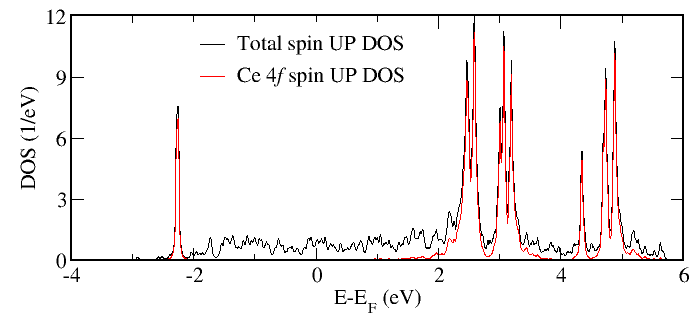
As one may clearly see, the Ce 4f band is split by the local Coulomb interaction into the filled lower Hubbard band and empty upper Hubbard band (the latter is additionally split into several peaks due to the Hund’s rule coupling and multiplet effects).