On the example of SrVO3 we will discuss now how to set up a full working calculation, including the initialization of the CTHYB solver. Some additional parameter are introduced to make the calculation more efficient. This is a more advanced example, which is also suited for parallel execution.
For the convenience of the user, we provide also a full
python script (dft_dmft_cthyb.py).
The user has to adapt it to his own needs. How to execute your script is described here.
The conversion will now be discussed in detail for the Wien2k and VASP packages. For more details we refer to the documentation.
DFT (Wien2k) and Wannier orbitals
DFT setup
First, we do a DFT calculation, using the Wien2k package. As main input file we have to provide the so-called struct file SrVO3.struct. We use the following:
SrVO3
P   LATTICE,NONEQUIV.ATOMS:  3221_Pm-3m
MODE OF CALC=RELA unit=bohr
  7.261300  7.261300  7.261300 90.000000 90.000000 90.000000
ATOM   1: X=0.00000000 Y=0.00000000 Z=0.00000000
          MULT= 1          ISPLIT= 2
Sr         NPT=  781  R0=0.00001000 RMT=   2.50000   Z: 38.0
LOCAL ROT MATRIX:    1.0000000 0.0000000 0.0000000
                     0.0000000 1.0000000 0.0000000
                     0.0000000 0.0000000 1.0000000
ATOM   2: X=0.50000000 Y=0.50000000 Z=0.50000000
          MULT= 1          ISPLIT= 2
V          NPT=  781  R0=0.00005000 RMT=   1.91      Z: 23.0
LOCAL ROT MATRIX:    1.0000000 0.0000000 0.0000000
                     0.0000000 1.0000000 0.0000000
                     0.0000000 0.0000000 1.0000000
ATOM  -3: X=0.00000000 Y=0.50000000 Z=0.50000000
          MULT= 3          ISPLIT=-2
      -3: X=0.50000000 Y=0.00000000 Z=0.50000000
      -3: X=0.50000000 Y=0.50000000 Z=0.00000000
O          NPT=  781  R0=0.00010000 RMT=   1.70      Z:  8.0
LOCAL ROT MATRIX:    0.0000000 0.0000000 1.0000000
                     0.0000000 1.0000000 0.0000000
                    -1.0000000 0.0000000 0.0000000
   0      NUMBER OF SYMMETRY OPERATIONS
Instead of going through the whole initialisation process, we can use
init -b -vxc 5 -numk 5000
This is setting up a non-magnetic calculation, using the LDA and 5000 k-points in the full Brillouin zone. As usual, we start the DFT self consistent cycle by the Wien2k script
run
Wannier orbitals
As a next step, we calculate localised orbitals for the t2g orbitals with dmftproj.
We create the following input file, SrVO3.indmftpr
3                ! Nsort
1 1 3            ! Mult(Nsort)
3                ! lmax
complex          ! choice of angular harmonics
1 0 0 0          ! l included for each sort
0 0 0 0          ! If split into ireps, gives number of ireps. for a given orbital (otherwise 0)
cubic            ! choice of angular harmonics
1 1 2 0          ! l included for each sort
0 0 2 0          ! If split into ireps, gives number of ireps. for a given orbital (otherwise 0)
01               !
0                ! SO flag
complex          ! choice of angular harmonics
1 1 0 0          ! l included for each sort
0 0 0 0          ! If split into ireps, gives number of ireps. for a given orbital (otherwise 0)
-0.11 0.14  0    ! lower energy window limit, upper energy window limit, mode (0,1,2)
Details on this input file and how to use dmftproj are described here.
To prepare the input data for dmftproj we first execute lapw2 with the -almd option
x lapw2 -almd
Then dmftproj is executed in its default mode (i.e. without spin-polarization or spin-orbit included)
dmftproj
This program produces the necessary files for the conversion to the hdf5 file structure. This is done using
the python module Wien2kConverter.
A simple python script that initialises the converter is:
from triqs_dft_tools.converters import Wien2kConverter
Converter = Wien2kConverter(filename = "SrVO3")
After initializing the interface module, we can now convert the input text files to the hdf5 archive by:
Converter.convert_dft_input()
This reads all the data, and stores everything that is necessary for the DMFT calculation in the file SrVO3.h5.
The DMFT calculation
The DMFT script itself is, except very few details, independent of the DFT package that was used to calculate the local orbitals. As soon as one has converted everything to the hdf5 format, the following procedure is practially the same.
Loading modules
First, we load the necessary modules:
from triqs_dft_tools.sumk_dft import *
from triqs.gfs import *
from h5 import HDFArchive
from triqs.operators.util import *
from triqs_cthyb import *
import triqs.utility.mpi as mpi
The last two lines load the modules for the construction of the CTHYB solver.
Initializing SumkDFT
We define some parameters, which should be self-explanatory:
dft_filename = 'SrVO3'          # filename
U = 4.0                         # interaction parameters
J = 0.65
beta = 40                       # inverse temperature
loops = 15                      # number of DMFT loops
mix = 0.8                       # mixing factor of Sigma after solution of the AIM
dc_type = 1                     # DC type: 0 FLL, 1 Held, 2 AMF
use_blocks = True               # use bloc structure from DFT input
prec_mu = 0.0001                # precision of chemical potential
And next, we can initialize the SumkDFT class:
SK = SumkDFT(hdf_file=dft_filename+'.h5',use_dft_blocks=use_blocks)
Initializing the solver
We also have to specify the CTHYB solver related settings. We assume that the DMFT script for SrVO3 is executed on 16 cores. A sufficient set of parameters for a first guess is:
p = {}
# solver
p["random_seed"] = 123 * mpi.rank + 567
p["length_cycle"] = 200
p["n_warmup_cycles"] = 100000
p["n_cycles"] = 1000000
# tail fit
p["perform_tail_fit"] = True
p["fit_max_moment"] = 4
p["fit_min_n"] = 30
p["fit_max_n"] = 60
# measure impurity density matrix to get self-energy moments for improved tail fit
p["measure_density_matrix"] = True
p["use_norm_as_weight"] = True
Here we use a tail fit to deal with numerical noise of higher Matsubara frequencies. For other options and more details on the solver parameters, we refer the user to the CTHYB solver documentation. It is important to note that the solver parameters have to be adjusted for each material individually. A guide on how to set the tail fit parameters is given below.
The next step is to initialize the
solver class.
It consist of two parts:
Calculating the multi-band interaction matrix, and constructing the interaction Hamiltonian.
Initializing the solver class itself.
The first step is done using methods of the TRIQS library:
n_orb = SK.corr_shells[0]['dim']
spin_names = ["up","down"]
# Use GF structure determined by DFT blocks:
gf_struct = SK.gf_struct_solver_list[0]
# Construct U matrix for density-density calculations:
Umat, Upmat = U_matrix_kanamori(n_orb=n_orb, U_int=U, J_hund=J)
We assumed here that we want to use an interaction matrix with Kanamori definitions of \(U\) and \(J\).
Next, we construct the Hamiltonian and the solver:
h_int = h_int_density(spin_names, n_orb, map_operator_structure=SK.sumk_to_solver[0], U=Umat, Uprime=Upmat)
S = Solver(beta=beta, gf_struct=gf_struct)
As you see, we take only density-density interactions into account. Other Hamiltonians with, e.g. with full rotational invariant interactions are:
h_int_kanamori
h_int_slater
For other choices of the interaction matrices (e.g Slater representation) or Hamiltonians, we refer to the reference manual of the TRIQS library.
As a last step, we initialize the subgroup in the hdf5 archive to store the results:
if mpi.is_master_node():
    with HDFArchive(dft_filename+'.h5') as ar:
        if (not ar.is_group('dmft_output')):
            ar.create_group('dmft_output')
DMFT cycle
Now we can go to the definition of the self-consistency step. It consists again of the basic steps discussed in the previous section, with some additional refinements:
for iteration_number in range(1,loops+1):
    if mpi.is_master_node(): print("Iteration = ", iteration_number)

    SK.symm_deg_gf(S.Sigma_iw,ish=0)                        # symmetrizing Sigma
    SK.set_Sigma([ S.Sigma_iw ])                            # put Sigma into the SumK class
    chemical_potential = SK.calc_mu( precision = prec_mu )  # find the chemical potential for given density
    S.G_iw << SK.extract_G_loc()[0]                         # calc the local Green function
    mpi.report("Total charge of Gloc : %.6f"%S.G_iw.total_density())

    # In the first loop, init the DC term and the real part of Sigma:
    if (iteration_number==1):
        dm = S.G_iw.density()
        SK.calc_dc(dm, U_interact = U, J_hund = J, orb = 0, use_dc_formula = dc_type)
        S.Sigma_iw << SK.dc_imp[0]['up'][0,0]

    # Calculate new G0_iw to input into the solver:
    S.G0_iw << S.Sigma_iw + inverse(S.G_iw)
    S.G0_iw << inverse(S.G0_iw)

    # Solve the impurity problem:
    S.solve(h_int=h_int, **p)

    # Solved. Now do post-solution stuff:
    mpi.report("Total charge of impurity problem : %.6f"%S.G_iw.total_density())

    # Now mix Sigma and G with factor mix, if wanted:
    if (iteration_number>1):
        if mpi.is_master_node():
            with HDFArchive(dft_filename+'.h5','r') as ar:
                mpi.report("Mixing Sigma and G with factor %s"%mix)
                S.Sigma_iw << mix * S.Sigma_iw + (1.0-mix) * ar['dmft_output']['Sigma_iw']
                S.G_iw << mix * S.G_iw + (1.0-mix) * ar['dmft_output']['G_iw']
        S.G_iw << mpi.bcast(S.G_iw)
        S.Sigma_iw << mpi.bcast(S.Sigma_iw)

    # Write the final Sigma and G to the hdf5 archive:
    if mpi.is_master_node():
        with HDFArchive(dft_filename+'.h5') as ar:
              ar['dmft_output']['iterations'] = iteration_number
              ar['dmft_output']['G_0'] = S.G0_iw
              ar['dmft_output']['G_tau'] = S.G_tau
              ar['dmft_output']['G_iw'] = S.G_iw
              ar['dmft_output']['Sigma_iw'] = S.Sigma_iw

    # Set the new double counting:
    dm = S.G_iw.density() # compute the density matrix of the impurity problem
    SK.calc_dc(dm, U_interact = U, J_hund = J, orb = 0, use_dc_formula = dc_type)

    # Save stuff into the user_data group of hdf5 archive in case of rerun:
    SK.save(['chemical_potential','dc_imp','dc_energ'])
This is all we need for the DFT+DMFT calculation. You can see in this code snippet, that all results of this calculation will be stored in a separate subgroup in the hdf5 file, called dmft_output. Note that this script performs 15 DMFT cycles, but does not check for convergence. Of course, it would be possible to build in convergence criteria. A simple check for convergence can be also done if you store multiple quantities of each iteration and analyse the convergence by hand. In general, it is advisable to start with a lower statistics (less measurements), but then increase it at a point close to converged results (e.g. after a few initial iterations). This helps to keep computational costs low during the first iterations.
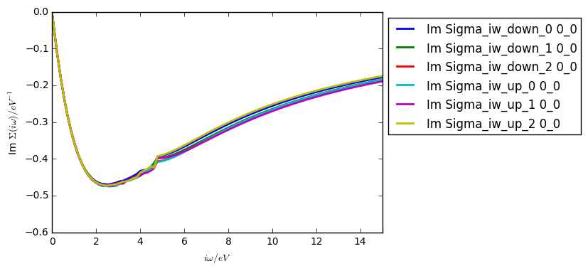
Using the Kanamori Hamiltonian and the parameters above (but on 16 cores), your self energy after the first iteration should look like the self energy shown below.
Tail fit parameters
A good way to identify suitable tail fit parameters is by “human inspection”. Therefore disabled the tail fitting first:
p["perform_tail_fit"] = False
and perform only one DMFT iteration. The resulting self energy can be tail fitted by hand:
Sigma_iw_fit = S.Sigma_iw.copy()
Sigma_iw_fit << tail_fit(S.Sigma_iw, fit_max_moment = 4, fit_min_n = 40, fit_max_n = 160)[0]
Plot the self energy and adjust the tail fit parameters such that you obtain a
proper fit. The fit_tail function is part
of the TRIQS library.
For a self energy which is going to zero for \(i\omega \rightarrow 0\) our suggestion is to start the tail fit (fit_min_n) at a Matsubara frequency considerable above the minimum of the self energy and to stop (fit_max_n) before the noise fully takes over. If it is difficult to find a reasonable fit in this region you should increase your statistics (number of measurements). Keep in mind that fit_min_n and fit_max_n also depend on \(\beta\).