Fitting data

A simple example

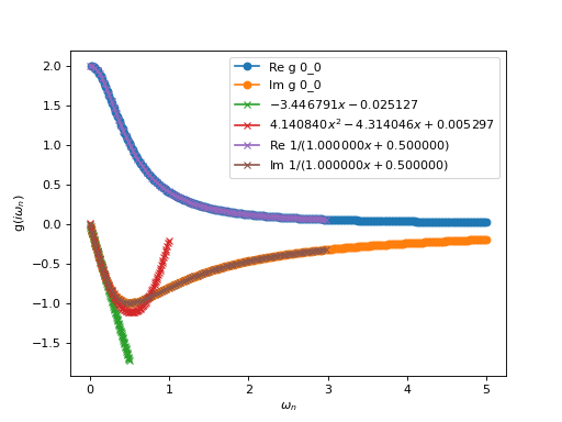
Let us for example fit the Green function :

from triqs.plot.mpl_interface import oplot
from triqs.gf import GfImFreq, Omega, inverse

g = GfImFreq(indices = [0], beta = 300, n_points = 1000, name = "g")
g << inverse( Omega + 0.5 )

# the data we want to fit...
# The green function for omega \in [0,0.2]
X,Y = g.x_data_view (x_window = (0,0.2), flatten_y = True )

from triqs.fit import Fit, linear, quadratic

fitl = Fit ( X,Y.imag, linear )
fitq = Fit ( X,Y.imag, quadratic )

oplot (g,     '-o', x_window = (0,5) )     
oplot (fitl , '-x', x_window = (0,0.5) )
oplot (fitq , '-x', x_window = (0,1) )

# a bit more complex, we want to fit with a one fermion level ....
# Cf the definition of linear and quadratic in the lib
one_fermion_level  =  lambda X, a,b   : 1/(a * X *1j  + b),    r"${1}/(%f x + %f)$"    , (1,1)

fit1 = Fit ( X,Y, one_fermion_level )
oplot (fit1 , '-x', x_window = (0,3) )

(Source code, png, hires.png, pdf)

Note that x_window appears in the x_data_view method to clip the data on a given window and in the plot function, to clip the plot itself.

Reference

The Fit class is very simple and is provided for convenience, but the reader is encouraged to have a look through it and adapt it (it is simply a call to scipy.leastsq).

class triqs.fit.Fit(x_array, y_array, fitter, p0=None)

A simple general functional fit of a X,Y plot

Given a function f(x, p0,p1,p2 …) with parameters p0, …, p2, and an init guess it adjust the parameters with least square method.

The fitting is done at construction

self.param is the tuple of adjusted parameters.

The object is callable : self(x) = f(x, *self.param), so it can be plotted e.g.

Example of fitfunc:

linear    =  lambda X, a,b  : a * X + b,             r"$%f x + %f$"          , (1,1)
quadratic =  lambda X, a,b,c: (a * X + b)*Omega + c, r"$%f x^2 + %f x + %f$" , (0,1,1)