Local Green’s functions
In this first part, we present a couple of examples in the form of a tutorial. The full reference is presented in the next sections.
A simple example
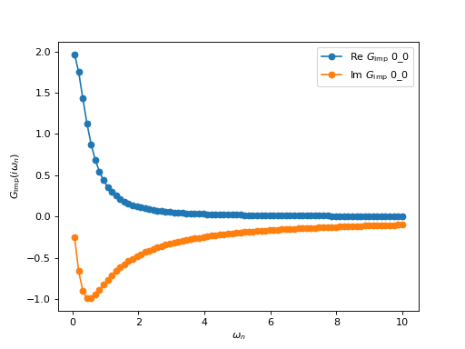
As a first example, we construct and plot the following Matsubara Green’s function:
This is done with the code :
# Import the Green's functions
from triqs.gf import GfImFreq, iOmega_n, inverse

# Create the Matsubara-frequency Green's function and initialize it
g = GfImFreq(indices = [1], beta = 50, n_points = 1000, name = "$G_\mathrm{imp}$")
g << inverse( iOmega_n + 0.5 )

from triqs.plot.mpl_interface import oplot
oplot(g, '-o',  x_window  = (0,10))
(Source code, png, hires.png, pdf)
In this very simple example, the Green’s function is just a 1x1 block. Let’s go through the different steps of the example:
# Import the Green's functions
from triqs.gf import GfImFreq, iOmega_n, inverse
This imports all the necessary classes to manipulate Green’s functions. In this example it allows
to use GfImFreq:
# Create the Matsubara-frequency Green's function and initialize it
g = GfImFreq(indices = [1], beta = 50, n_points = 1000, name = "$G_\mathrm{imp}$")
This creates a block Green’s function which has just one index
(1). beta is the inverse temperature, n_points is the number of
Matsubara frequencies.
g << inverse( iOmega_n + 0.5 )
This initializes the block with \(1/(i \omega_n + 0.5)\). Two points are worth noting here:
The right hand side (RHS) of this statement is a lazy expression: its evaluation is delayed until it is needed to fill the Green function.
The funny << operator means “set from”. It fills the Green function with the evaluation of the expression at the right.
oplot(g, '-o', x_window = (0,10))
These lines plot the block Green’s function (both the real and imaginary parts) using the matplotlib plotter. More details can be found in the section Plotting TRIQS objects.
A slightly more complicated example
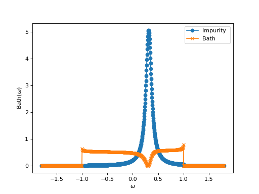
Let’s turn to another example. This time we consider a problem of a d-impurity level embedded in a flat conduction bath \(\Delta\) of s-electrons. We want to construct the corresponding 2x2 Green’s function:
This is done with the code:
from triqs.gf import GfReFreq, Omega, Wilson, inverse
import numpy

eps_d,t  = 0.3, 0.2

# Create the real-frequency Green's function and initialize it
g = GfReFreq(indices = ['s','d'], window = (-2, 2), n_points = 1000, name = "$G_\mathrm{s+d}$")
g['d','d'] = Omega - eps_d
g['d','s'] = t
g['s','d'] = t
g['s','s'] = inverse( Wilson(1.0) )
g.invert()

# Plot it with matplotlib. 'S' means: spectral function ( -1/pi Imag (g) )
from triqs.plot.mpl_interface import oplot, plt
oplot( g['d','d'], '-o', mode = 'S', x_window  = (-1.8,1.8), name = "Impurity" )
oplot( g['s','s'], '-x', mode = 'S', x_window  = (-1.8,1.8), name = "Bath" )
plt.show()
(Source code, png, hires.png, pdf)
Again, the Green’s function is just one block, but this time it is a 2x2 block with off-diagonal elements. Another difference is that we use real-frequency Green’s functions in this example:
# Create the real-frequency Green's function and initialize it
g = GfReFreq(indices = ['s','d'], window = (-2, 2), n_points = 1000, name = "$G_\mathrm{s+d}$")
In this constructor for the block Green’s function, we specify that there are two indices s and d.
Because it is a real-frequency Green’s function we need to define the mesh on which it is
computed. This is done with the window and n_points options.
g['d','d'] = Omega - eps_d
g['d','s'] = t
g['s','d'] = t
g['s','s'] = inverse( Wilson(1.0) )
These lines initialize specific entries of the block Green’s function. Note how the elements are
accessed with [index1,index2]. These lines also show how to initialize a Green’s function
to a constant or to the inverse of a Flat bath (constant spectral function on an interval \([-D,D]\), with
\(D=1.0\) in our example).
g.invert()
invert() inverts the entire block Green’s function (as a matrix).
# Plot it with matplotlib. 'S' means: spectral function ( -1/pi Imag (g) )
from triqs.plot.mpl_interface import oplot, plt
oplot( g['d','d'], '-o', mode = 'S', x_window  = (-1.8,1.8), name = "Impurity" )
oplot( g['s','s'], '-x', mode = 'S', x_window  = (-1.8,1.8), name = "Bath" )
Here, we isolate some elements of the blocks Green’s function. It is also the first example of an operation on the block Green’s function, which is multiplied by a scalar. The last lines of the script just plot these new objects.