Continuation of matrix-valued functions [1]
In principle one can perform the analytic continuation separately for each matrix element,
using the conventional entropy for diagonal elements and the modified entropy for the off-diagonals.
We term this way of dealing with matrix-valued Green function ElementwiseMaxEnt.
Using, e.g., a flat default model for each element reflects the total absence of previous knowledge on the problem. However, we know that a necessary condition for the positive semi-definiteness of the resulting spectral function matrix is
For example, for a problem where all diagonal elements of the spectral function are zero at a certain frequency \(\omega\), this condition implies that also all off-diagonal elements have to be zero at this \(\omega\). Thus, once the diagonal elements have been analytically continued, this condition constitutes additional knowledge about the problem which can be incorporated by choosing a default model for the off-diagonal elements \(D_{ll'}(\omega)\) accordingly,
Here, \(\epsilon\) is a small number to prevent the default model from becoming zero, so that no
division by zero occurs in the entropy term. We call this approach PoormanMaxEnt.
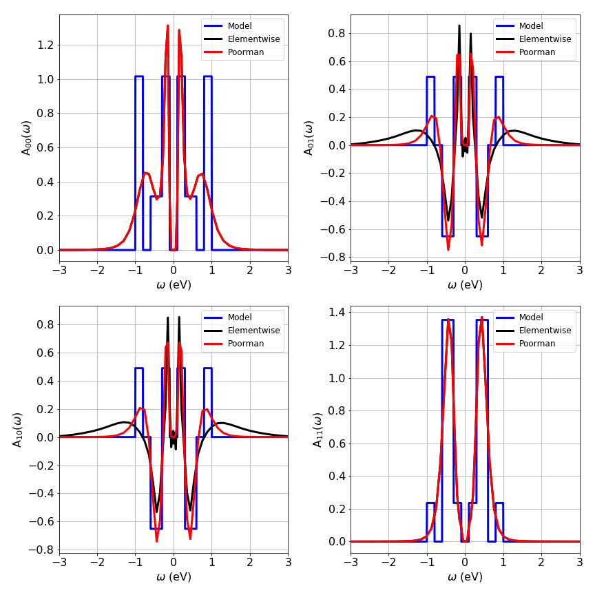
The example below shows the continuation of 2x2 model Green function. The special choice of the default model does indeed improve the results of the off-diagonal elements. However, for physical systems, the resulting spectral function matrix has to be positive semi-definite and Hermitian, which is usually not the case when the analytic continuation is carried out separately for each matrix element. Using the Poorman scheme usually improves the solution, but the only way to ensure that the obtained spectral function is indeed positive semi-definite and Hermitian is by treating the spectral function matrix as a whole. We plan to make the FullMatrixMaxEnt public in the future.
Example
An example for a 2x2 matrix:
 1
 2from triqs_maxent import *
 3
 4# Generate a 2x2 model Green function
 5#####################################
 6# TRIQS Green functions
 7G_iw = GfImFreq(beta=300, indices=[0, 1], n_points=200)
 8G_w = GfReFreq(indices=[0, 1], window=(-10, 10), n_points=5000)
 9
10# Initialize Green functions with a set of rectangles
11G_iw[1, 1] << (Flat(0.6) - Flat(0.3) / 2.0) * 2.0
12G_iw[0, 0] << ((Flat(0.3) - Flat(0.1) / 3.0) * 6.0 / 2.0 +
13               (Flat(1.0) - Flat(0.8) / (10.0 / 8.0)) * 2.0 * 10.0 / 2.0) / 4.0
14G_w[1, 1] << (Flat(0.6) - Flat(0.3) / 2.0) * 2.0
15G_w[0, 0] << ((Flat(0.3) - Flat(0.1) / 3.0) * 6.0 / 2.0 +
16              (Flat(1.0) - Flat(0.8) / (10.0 / 8.0)) * 2.0 * 10.0 / 2.0) / 4.0
17
18# Rotation to generate off-diagonals
19theta = np.pi / 7
20R = np.array([[np.cos(theta), -np.sin(theta)], [np.sin(theta), np.cos(theta)]])
21G_iw_rot = copy.deepcopy(G_iw)
22G_iw_rot.from_L_G_R(R, G_iw, R.transpose())
23G_w_rot = copy.deepcopy(G_w)
24G_w_rot.from_L_G_R(R, G_w, R.transpose())
25
26# Calculate G(tau) and add some noise
27G_tau_rot = GfImTime(beta=G_iw_rot.beta, indices=G_iw_rot.indices)
28G_tau_rot.set_from_fourier(G_iw_rot)
29G_tau_rot.data[:, :, :] = G_tau_rot.data.real + 1.e-4 * np.reshape(
30    np.random.randn(np.size(G_tau_rot.data)),
31    np.shape(G_tau_rot.data))
32
33# Run Elementwise and Poorman MaxEnt
34####################################
35
36# Elementwise (all elements individually)
37ew = ElementwiseMaxEnt(use_hermiticity=True)
38ew.set_G_tau(G_tau_rot, tau_new=np.linspace(0, G_iw_rot.beta, 200))
39ew.set_error(1e-4)
40result_ew = ew.run()
41
42# Poorman (construct default model for off-diagonals from diagonal solution)
43pm = PoormanMaxEnt(use_hermiticity=True)
44pm.set_G_tau(G_tau_rot, tau_new=np.linspace(0, G_iw_rot.beta, 200))
45pm.set_error(1.e-4)
46result_pm = pm.run()
47
48
49# Plot resulting spectra
50########################
51import matplotlib
52matplotlib.rcParams['figure.figsize'] = (12, 12)
53matplotlib.rcParams.update({'font.size': 16})
54from triqs.plot.mpl_interface import oplot
55
56fig = plt.figure()
57for i in range(G_iw_rot.N1):
58    for j in range(G_iw_rot.N2):
59        plt.subplot(2, 2, i * 2 + j + 1)
60        oplot(G_w_rot[i, j], mode='S', color='b', lw=3, label='Model')
61        plt.plot(result_ew.omega,
62                 result_ew.get_A_out('LineFitAnalyzer')[i][j],
63                 'k', lw=3, label='Elementwise')
64        plt.plot(result_pm.omega,
65                 result_pm.get_A_out('LineFitAnalyzer')[i][j],
66                 'r', lw=3, label='Poorman')
67        plt.xlim(-3, 3)
68        plt.ylabel(r'A$_{%s%s}$($\omega$)' % (i, j))
69        plt.xlabel(r'$\omega$ (eV)')
70        plt.grid()
71        plt.legend(loc='upper right', prop={'size': 12})
72
73# Interactive Visualization in Jupyter Notebook
74###############################################
75
76from triqs_maxent.plot.jupyter_plot_maxent import JupyterPlotMaxEnt
77JupyterPlotMaxEnt(result_pm)
Note
This model with very sharp edges is a complicated case for the Maximum Entropy method; it tends to smoothen them out considerably. However, the obtained curves show roughly the quality of the results that can be obtained with MaxEnt. After all, the analytic continuation is an ill-posed problem. For a given \(G(\tau)\) (with noise) one can find infinitely many \(A(\omega)\) to satisfy the data within the given error bars. The comparision of the original (sharp) spectral function to the MaxEnt \(A(\omega)\) demonstrates the accuracy of analytic continuations: The overall structure and features are reproduced, but details are smeard out (especially at higher frequencies). In any case, one cannot expect that \(A_i(\omega)\to G(\tau) \to A_c(\omega\)) results in \(A_i(\omega) = A_c(\omega)\).
Footnotes