Real-material application: SrVO₃

In this example we perform an analytic continuation for an impurity \(G(\tau)\) calculated from DFT+DMFT for the t_2g subspace of paramagnetic SrVO₃. All three t_2g orbitals are degenerate, thus we have to perform the continuation only for one orbital. The DFT+DMFT solution itself can be obtained with the TRIQS/dft_tools package and we like to refer the interested user to the corresponding user guide page on SrVO₃. However, for this example we directly provide the \(G(\tau)\) at \(\beta = 37.5~1/eV\) as a downloadable file. For simplicity we use a constant error of \(10^{-3}\) for all \(\tau\) points.

Running TauMaxEnt

from triqs_maxent import *
import numpy as np

# initialize TauMaxEnt, set G_tau from file, set omega and alpha mesh
# set the probability; then add Bryan and Classic analyzers are added by the program
# LineFit and Chi2Curvature analyzers are set set by default
tm = TauMaxEnt(probability='normal')
tm.set_G_tau_file(filename='srvo3_G_tau.dat', tau_col=0, G_col=1, err_col=2)
tm.omega = HyperbolicOmegaMesh(omega_min=-10, omega_max=10, n_points=400)
tm.alpha_mesh = LogAlphaMesh(alpha_min=1e-4, alpha_max=100, n_points=50)
# run MaxEnt
res = tm.run()

# run the same calculation with preblur
# Here we guess the preblur parameter b, but it is better to determine
# b with a chi2(b) linefit or curvature analysis!
# set preblur parameter b, PreblurA_of_H and PreblurKernel
b = 0.1
tm.A_of_H = PreblurA_of_H(b=b, omega=tm.omega)
K_orig = tm.K
tm.K = PreblurKernel(K=K_orig, b=b)
# run Maxent with preblur
res_pb = tm.run()

Analyzing the result

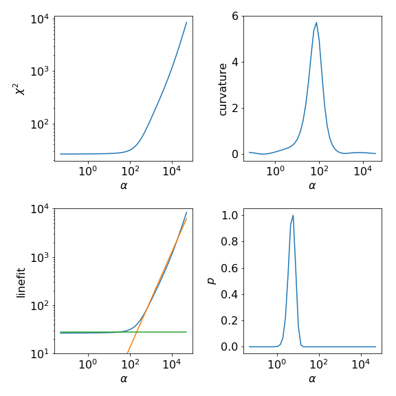
In the following we plot \(\chi^2(\alpha)\) and the corresponding curvature as well as the result of the linefit. The LineFitAnalyzer uses as optimal \(\alpha\) value the intersection of the two fitted lines. The Chi2CurvatureAnalyzer uses the \(\alpha\) at the maximum curvature of \(\chi^2(\alpha)\). Further we enabled in this example the calculation of the probability for each \(\alpha\). Then, the ClassicAnalyzer takes the \(\alpha\) at the maximum of the probability and the BryanAnalyzer averages over all spectral functions weighted by the corresponding probabilities.

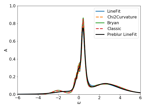
Usually the results of the LineFitAnalyzer and the Chi2CurvatureAnalyzer are similar. Also, as the probability is often sharply peaked at an \(\alpha\) value the ClassicAnalyzer and BryanAnalyzer give similar spectral functions.

# analysis of the output (here we only look at the normal run without preblur)
import matplotlib.pyplot as plt
plt.rcParams['figure.figsize'] = (8, 8)
plt.rcParams.update({'font.size': 16})

fig1 = plt.figure()
# chi2(alpha)
plt.subplot(2, 2, 1)
res.plot_chi2()
# curvature(alpha)
plt.subplot(2, 2, 2)
res.analyzer_results['Chi2CurvatureAnalyzer'].plot_curvature()
# linefit of chi2(alpha)
plt.subplot(2, 2, 3)
res.analyzer_results['LineFitAnalyzer'].plot_linefit()
plt.ylim(1e1, 1e4)
# probablity(alpha)
plt.subplot(2, 2, 4)
res.plot_probability()
plt.tight_layout()
fig1.savefig('srvo3_analysis.png')

# spectral function A
matplotlib.rcParams['figure.figsize'] = (8, 6)
fig2 = plt.figure()
plt.plot(res.omega, res.get_A_out('LineFitAnalyzer'),
         '-', lw=3, label='LineFit')
plt.plot(res.omega, res.get_A_out('Chi2CurvatureAnalyzer'),
         '--', lw=3, label='Chi2Curvature')
plt.plot(res.omega, res.get_A_out('BryanAnalyzer'),
         '-', lw=3, label='Bryan')
plt.plot(res.omega, res.get_A_out('ClassicAnalyzer'),
         '--', lw=3, label='Classic')
plt.plot(res_pb.omega, res_pb.get_A_out('LineFitAnalyzer'),
         'k-', lw=3, label='Preblur LineFit')
plt.legend()
plt.xlim(-6, 6)
plt.ylim(0, 1)
plt.ylabel('A')
plt.xlabel(r'$\omega$')
plt.tight_layout()
fig2.savefig('srvo3_A.png')

# print the optimal alpha-values
print(('Curvature: ', res.analyzer_results[
      'Chi2CurvatureAnalyzer']['alpha_index']))
print(('LineFit: ', res.analyzer_results['LineFitAnalyzer']['alpha_index']))
print(('Classic: ', res.analyzer_results['ClassicAnalyzer']['alpha_index']))
print(('Preblur LineFit: ', res_pb.analyzer_results[
      'LineFitAnalyzer']['alpha_index']))

Note that the LineFitAnalyzer and the Chi2CurvatureAnalyzer are less sensitive to the given error, and thus work also well when the real error is not known. On the other hand, the analyzers based on the probability depend on the given error. As an exercise try to set the error to a different value, e.g.:

tm.error(1e-4)

and compare the result spectral functions of the different analyzers. You might need to adjust also the \(\alpha\)-grid. If the error is, e.g., scaled by a factor of 10, the \(\alpha\) range should be changed by a factor of 100.

Visualization in notebook

Above we have used the plot_* method, which is implemented for many objects, to visualize the output. However, the data can be also visualized with the interactive Jupyter widget JupyterPlotMaxEnt:

from triqs_maxent.plot.jupyter_plot_maxent import JupyterPlotMaxEnt
JupyterPlotMaxEnt(res)

For further ways to visualize your results have a look at the Visualization page.

Saving the data to a h5-file

The data of the MaxEnt run (MaxEntResult) can be stored as MaxEntResultData object to a h5-file with:

from h5 import *
with HDFArchive('srvo3_maxent.h5','w') as ar:
    ar['maxent_result'] = res.data
    ar['maxent_result_pb'] = res_pb.data