Continuation of metallic solutions using preblur

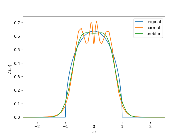
The MaxEnt formalism has the tendency of producing spurious noise around the \(\omega=0\) point. This is usually not problematic for insulating solutions, but not desirable for metallic spectral functions.

One strategy to tackle this is the so-called preblur technique [1]. There, a so-called hidden image \(H\) is introduced, with the spectral function being \(A = B H\) [2]. The matrix \(B\) is the blur matrix; multiplying by \(B\) is equal to a convolution with a Gaussian (its width \(b\) is an external parameter). Then, in the cost function, both \(H\) and \(A\) are used,

\[Q_{\alpha}(v) = \frac12 \chi^2(A(H(v))) - \alpha S(H(v)).\]

The parametrization \(H(v)\) is, e.g., Bryan’s parametrization, \(H(v) = D e^{Vv}\). The parametrization \(A(H)\) is, of course, \(A = B H\).

The class MaxEntCostFunction accepts a parameter A_of_H. Only two different parametrizations for \(A(H)\) are implemented: the IdentityA_of_H and PreblurA_of_H variants. The former just chooses the usual \(A(H) = H\), the latter uses \(A(H) = BH\) as discussed here.

Note that, for performance reasons, the kernel has to be redefined to include the blur matrix. This is done by choosing the PreblurKernel.

The calculation should be performed using different values for \(b\). The best value of \(b\) can be determined similarly to determining \(\alpha\); e.g., by calculating the probability of every \(b\) or by looking at \(\log(\chi^2)\) of \(\log b\).

Example

A full example:

from triqs_maxent.analyzers.linefit_analyzer import fit_piecewise

try:
    # TRIQS 2.1
    from triqs.gf import *
    GfImFreq
except NameError:
    # TRIQS 1.4
    from triqs.gf.local import *
from triqs_maxent import *
from triqs_maxent.analyzers.linefit_analyzer import fit_piecewise

# whether we want to save and plot the results
save = False
plot = True

# construct a test Green function
# for reference, G(w)
G_w = GfReFreq(window=(-3, 3), indices=[0])
G_w << SemiCircular(1)

# the G(iw)
G_iw = GfImFreq(beta=40, indices=[0], n_points=50)
G_iw << SemiCircular(1)

# we inverse Fourier-transform G(iw) to G(tau)
G_tau = GfImTime(beta=G_iw.beta, indices=[0], n_points=102)
G_tau.set_from_fourier(G_iw)
# and add some noise (MaxEnt does not work without noise)
G_tau.data[:, 0, 0] = G_tau.data[:, 0, 0] + \
    1.e-4 * np.random.randn(len(G_tau.data))

tm = TauMaxEnt()
# the following allows to Ctrl-C the calculation and choose what to do
tm.interactive = True
tm.set_G_tau(G_tau)
# set an appropriate alpha mesh
tm.alpha_mesh = LogAlphaMesh(alpha_min=0.08, alpha_max=1000, n_points=30)
tm.set_error(1.e-4)

# run without preblur
result_normal = tm.run()
last_result = result_normal

K_tau = tm.K

# loop over different values of the preblur parameter b
results_preblur = {}
for b in [0.05, 0.1, 0.15, 0.2, 0.25, 0.3, 0.4]:
    print('Running for b = {}'.format(b))
    tm.A_of_H = PreblurA_of_H(b=b, omega=tm.omega)
    tm.K = PreblurKernel(K=K_tau, b=b)
    # initialize A(w) with the last result, this leads to faster convergence
    tm.A_init = last_result.analyzer_results['LineFitAnalyzer']['A_out']
    results_preblur[b] = tm.run()
    last_result = results_preblur[b]

# save the results
if save:
    from h5 import HDFArchive
    with HDFArchive('preblur.h5', 'w') as ar:
        ar['result_normal'] = result_normal.data
        ar['results_preblur'] = [r.data for r in results_preblur]

# extract the chi2 value from the optimal alpha for each blur parameter
chi2s = []
# we have to reverse-sort it because fit_piecewise expects it in that order
b_vals = sorted(list(results_preblur.keys()), reverse=True)
for b in b_vals:
    r = results_preblur[b]
    alpha_index = r.analyzer_results['LineFitAnalyzer']['alpha_index']
    chi2s.append(r.chi2[alpha_index])

# perform a linefit to get the optimal b value
b_index, _ = fit_piecewise(np.log10(b_vals), np.log10(chi2s))
b_ideal = b_vals[b_index]
print('Ideal b value = ', b_ideal)

if plot:
    import matplotlib.pyplot as plt
    from triqs.plot.mpl_interface import oplot
    oplot(G_w, mode='S')
    result_normal.analyzer_results['LineFitAnalyzer'].plot_A_out()
    results_preblur[b_ideal].analyzer_results['LineFitAnalyzer'].plot_A_out()
    plt.xlabel(r'$\omega$')
    plt.ylabel(r'$A(\omega)$')
    plt.legend(['original', 'normal', 'preblur'])
    plt.xlim(-2.5, 2.5)
    plt.savefig('preblur_A.png')
    plt.show()

Footnotes

[1]

J. Skilling, Fundamentals of MaxEnt in data analysis, in Maximum Entropy in Action, edited by B.Buck and V.A. Macaulay (Clarendon Press, Oxford, UK, 1991), p. 19.

[2]

As a slight complication, for non-uniform \(\omega\) meshes, we have \(A = B H /\Delta \omega\) and \(G_{rec} = K \Delta \omega B H\), where \(H\) contains a \(\Delta\omega\) (i.e. the hidden image itself would be \(H/\Delta\omega\)).