Continuation of a 1x1 Green Function

For continuing a single diagonal element of a Green function, the TauMaxEnt class is the right tool. The Green function can be given as GfImTime (use set_G_tau()) or as GfImFreq (use set_G_iw()). Additionally, it is possible to set \(G(\tau)\) directly with a data array (set_G_tau_data()) or load it from a file (set_G_tau_file()).

Creation of a mock \(G(\tau)\)

For the following guide, we will assume that you have a TRIQS GfImTime ready; if you have not, you can produce one, for example an insulating mock \(G(\tau)\), using

#TRIQS 2.1
from triqs.gf import *
#TRIQS 1.4
from triqs.gf.local import *
import numpy as np

err = 1.e-5
G_iw = GfImFreq(beta=10, indices=[0])
G_w = GfReFreq(window=(-10, 10), indices=[0])
G_iw << SemiCircular(1)-0.5*SemiCircular(0.5)
G_w << SemiCircular(1)-0.5*SemiCircular(0.5)
G_tau = GfImTime(beta=10, indices=[0], n_points=2501)
G_tau.set_from_fourier(G_iw)
G_tau.data[:, 0, 0] += err * np.random.randn(len(G_tau.data))

Here, we added random Gaussian noise to the \(G(\tau)\). From experience, we know that the MaxEnt algorithm does not work well with exact data, we thus have to have some kind of noise on the data.

Setting up and running TauMaxEnt

The class to analytically continue a \(G(\tau)\) is the TauMaxEnt class. It sets up everything we need; but internally, the work is done by the MaxEntLoop class.

In MaxEnt, we minimize the functional (cost function)

\[Q[A; \alpha] = \frac12 \chi^2[A, G(\tau), \sigma] - \alpha S[A, D].\]

The ingredients are the spectral function \(A\), the data \(G(\tau)\), the error \(\sigma\), the default model \(D\) and the hyper-parameter \(\alpha\).

This cost function is represented by the CostFunction class. There are two different versions of the MaxEnt cost function available, one very general one, the MaxEntCostFunction, and one version with some optimizations for the one-orbital case [1], which is called BryanCostFunction [2]. Here, the latter is the right choice.

The MaxEntCostFunction is used by default, but we can tell the TauMaxEnt class to use the BryanCostFunction with TauMaxEnt(cost_function=BryanCostFunction()) or TauMaxEnt(cost_function='bryan') in its constructor.

We then have to set the data \(G(\tau)\). As we have a TRIQS GfImTime we do this with set_G_tau() Furthermore, we have to set the error \(\sigma\). If you have a covariance matrix available you can set it with set_cov(). In our case, we just added random noise to \(G(\tau)\), thus we can use the method set_error(). Note that a \(\tau\) dependent error is possible by passing a vector.

The default model is chosen to be flat by default. The hyper-parameter \(\alpha\) will be varied in a loop; for many cases, the default setting should be okay (see below for adjusting the \(\alpha\) range).

Note that the calculation of probabilities is not enabled by default. You can achieve this by setting TauMaxEnt(probability=NormalLogProbability()) or TauMaxEnt(probability='normal') (see also Probabilities).

Then, the MaxEnt procedure can be started using run(). It returns the result as a MaxEntResult object.

from triqs_maxent import *

tm = TauMaxEnt(cost_function='bryan', probability='normal')
tm.set_G_tau(G_tau)
tm.set_error(10*err)
result = tm.run()

Here, we used tm.set_error(10*err) as given error - we will come back to this in the discussion of the results.

If you set tm.interactive to True (the default value), by pressing Ctrl+C, you can choose from several different options how to proceed, e.g., just aborting the minimization of the current \(\alpha\), aborting the \(\alpha\) loop, or exiting right away.

Finally, we save the result to a h5-file with

from h5 import HDFArchive

with HDFArchive('file_name.h5','w') as ar:
    ar['maxent'] = result.data

Changing some of the parameters

The \(\alpha\) mesh can be changed with tm.alpha_mesh; an example would be

tm.alpha_mesh = LogAlphaMesh(alpha_min=0.01, alpha_max=2000, n_points=60)

Often, it can be useful to adjust the \(\omega\) mesh (see omega meshes). It can be set, e.g., using

tm.omega = HyperbolicOmegaMesh(omega_min=-10, omega_max=10, n_points=101)

The default model can be changed by assigning it to tm.D.

Choosing the value of the hyper-parameter

There are several methods to choose the final spectral function given all the spectral functions that minimize the cost function Q for the different values of \(\alpha\) (see also Ways to choose alpha).

In the code, this is done using so-called analyzers (see Analyzer). The variable tm.analyzers contains a list of analyzer class instances; the result is analyzed with each of them. By default, the LineFitAnalyzer, the Chi2CurvatureAnalyzer and the EntropyAnalyzer are used. Should you have enabled the probabilities, the BryanAnalyzer and the ClassicAnalyzer are added automatically.

Note that the LineFitAnalyzer and the Chi2CurvatureAnalyzer, which are based on the analysis of the function \(\log(\chi^2)\) versus \(\log(\alpha)\), are not very sensitive to the given error (if constant), as scaling the error will just result in a shift of the chosen \(\alpha\). On the other hand, the chosen \(\alpha\) in the probabilistic methods depends strongly on the given error. This is the reason why we scaled the given error by a factor of 10 for the example above, as otherwise it would result in a severe over-fitting of the data (too small \(\alpha\)), see also [3] [4].

Let’s turn back to the output of the analyzers. Each analyzer produces one single spectral function, which can be accessed, e.g. for the LineFitAnalyzer, as

result.get_A_out('LineFitAnalyzer')

As the LineFitAnalyzer is the default, it is also possible to just use result.A_out or result.get_A_out().

Some important information on the performance of the analyzer is available as well; it can be found by getting the analyzer result as:

result.analyzer_results['LineFitAnalyzer'][attribute]

where attribute can be, e.g., 'A_out' (the same as above). In addition to the attribute A_out, the AnalyzerResult also contains a name (which is also how it is addressed in result.analyzer_results), an info field containing human-readable information about which \(\alpha\) the analyzer chooses, and some analyzer-dependent fields.

Visualizing and checking the results

For a summary of visualization tools see the Visualization page.

The following script and the figures show the most important things you should look at after your MaxEnt run (however, in practice it might be easier to just use plot_maxent or JupyterPlotMaxEnt as described in the Visualization page). Again, these plots are for the example given above.

A short description on how the results of the analyzers should be checked is also provided in the reference guide for the Analyzers.

from triqs.plot.mpl_interface import oplot

fig1 = plt.figure()
# chi2(alpha) and linefit
plt.subplot(2, 2, 1)
res.analyzer_results['LineFitAnalyzer'].plot_linefit()
res.plot_chi2()
plt.ylim(1e1, 1e3)
# curvature(alpha)
plt.subplot(2, 2, 3)
res.analyzer_results['Chi2CurvatureAnalyzer'].plot_curvature()
# probablity(alpha)
plt.subplot(2, 2, 2)
res.plot_probability()
# backtransformed G_rec(tau) and original G(tau)
# by default (plot_G=True) also original G(tau) is plotted
plt.subplot(2, 2, 4)
res.plot_G_rec(alpha_index=5)
plt.tight_layout()

# spectral function A
fig2 = plt.figure()
oplot(G_w, mode='S', color='k', lw=3, label='Original Model')
plt.plot(res.omega, res.analyzer_results['LineFitAnalyzer']['A_out'],
         '-', lw=3, label='LineFit')
plt.plot(res.omega, res.analyzer_results['Chi2CurvatureAnalyzer']['A_out'],
         '--', lw=3, label='Chi2Curvature')
plt.plot(res.omega, res.analyzer_results['BryanAnalyzer']['A_out'],
         '-', lw=3, label='Bryan')
plt.plot(res.omega, res.analyzer_results['ClassicAnalyzer']['A_out'],
         '--', lw=3, label='Classic')

plt.legend()
plt.xlim(-3, 3)
plt.ylim(0, 0.6)
plt.ylabel('A')
plt.xlabel(r'$\omega$')
plt.tight_layout()

# print the optimal alpha-values
print(('Curvature: ',
      res.analyzer_results['Chi2CurvatureAnalyzer']['alpha_index']))
print(('LineFit: ', res.analyzer_results['LineFitAnalyzer']['alpha_index']))
print(('Classic: ', res.analyzer_results['ClassicAnalyzer']['alpha_index']))

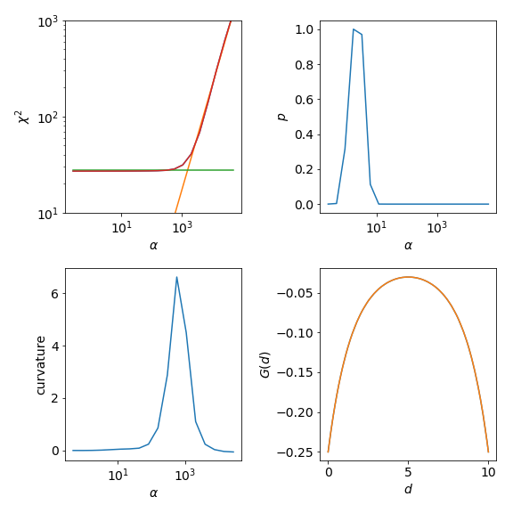
The upper left graph shows \(\chi^2\) and the characteristic kink separating the noise-fitting regime form the information-fitting regime. If this is not the case in your own calculation you need to adjust your \(\alpha\) range. For even higher \(\alpha\) one would enter the default-regime the default model is reproduced. There \(\chi^2\) becomes flat again.

The LineFitAnalyzer fits two straight lines to the \(\chi^2\) curve and their intersection determines the optimal \(\alpha\). The Chi2CurvatureAnalyzer calculates the curvature of the \(\chi^2\) curve and selects the point of maximum curvature. This is shown in the lower left graph. Usually, the optimal \(\alpha\) of these two analyzers is very similar, but the LineFitAnalyzer tends to be more stable in difficult cases were multiple maxima are present in the curvature.

The upper right graph shows the probability. The ClassicAnalyzer selects the \(\alpha\) at the maximum of the probability and the BryanAnalyzer averages over all spectral functions weighted with their respective probabilities. As the probability is usually sharply peaked around the optimal \(\alpha\) the results of these two analyzers are often very similar. However, the location of the maximum is sensitive to the given error \(\sigma\).

Finally, the lower right graph show the original \(G(\tau)\) compared to the reconstructed \(G_{rec}(\tau)\) for alpha_index=5. This is the index selected by the LineFitAnalyzer.

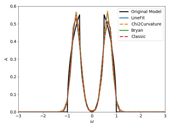
For this specific example the resulting spectral functions are rather similar, but don’t forget that we have used a factor of ten in the given error to prevent the probabilistic analyzers from over-fitting the data.

Metallic Model

As an exercise you can try to perform the analytic continuation for a (metallic) semi-circular spectral function with G_iw << SemiCircular(1.0). You will observe that the MaxEnt spectral functions will tend to oscillate around zero. One way to suppress these oscillations is the preblur method; further described here.

Footnotes