Continuation of self-energies: Sr₂RuO₄

A central quantity of many-body theory is the self-energy \(\Sigma\). Often it is beneficial to perform the analytic continuation for the self-energy instead of the Green function. Different ways to continue self-energies exist (see Ref. [1]), but the most commonly used approach is to continue an auxiliary quantity \(G_{aux}(\omega)\). This requires the following five steps:

construction of \(G_{aux}(i\omega_n)\) from the self-energy \(\Sigma(i\omega_n)\),

inverse Fourier transform to \(G_{aux}(\tau)\)

analytic continuation of \(G_{aux}(\tau)\) to \(A_{aux}(\omega)\),

construction of \(G_{aux}(\omega+i0^+)\) from \(A_{aux}(\omega)\),

and calculating \(\Sigma(\omega+i0^+)\) from \(G_{aux}(\omega+i0^+)\).

Beside the analytic continuation itself the above steps are carried out by the SigmaContinuator. This tool has two possible constructions of \(G_{aux}\) implemented:

DirectSigmaContinuator: \(G_{aux}(z) = \Sigma(z) - \Sigma(i\infty)\) where \(\Sigma(i\infty)\) is the constant term of the high-frequency expansion of \(\Sigma(i\omega_n)\). For matrix-valued Green functions the resulting quantity \(G_{aux}\) would not obey the correct analytic high-frequency behavior. Therefore, the DirectSigmaContinuator is only implemented for the diagonal problems.

InversionSigmaContinuator: \(G_{aux}(z) = (z + C - \Sigma(z))^{-1}\) The constant \(C\) is a free parameter, but is usually set to \(C= \Sigma(i\infty) + \mu\) with the chemical potential \(\mu\) in DMFT calculations.

Note that an error propagation from \(\Sigma(i\omega_n)\) to \(G_{aux}(\tau)\) is currently not implemented in the SigmaContinuator.

The SigmaContinuator does accept TRIQS Green functions, but can be also used directly with TRIQS BlockGFs. How this is used in practise is shown in the example below.

Example

In the example below we continue the t_2g self-energy of Sr₂RuO₄ with the InversionSigmaContinuator. The self-energy is the result of a DFT+DMFT calculation performed at an inverse temperature \(\beta = 37.5~1/eV\) (h5-file).

After loading the self-energy we initialize the InversionSigmaContinuator isc with the constant shift C set to the double counting (dc). The SigmaContinuator directly takes a TRIQS Block Green function and calculates the auxiliary Green function \(G_{aux}(i\omega_n)\). We need to run six analytic continuations (for each block individually) by looping over all orbitals/spins of isc.Gaux_iw. In principle it would be sufficient to perform two continuations, because the t_2g-subspace consists of the xy and the degenerate xz/yz orbitals. Note that the self-energy in the h5-file is already symmetrized. We collect the results in the dict res and save it to the h5-file. Additionally, we save the SigmaContinuator.

from triqs_maxent import *
from h5 import *

# Load self-energy from h5-file
with HDFArchive('Sr2RuO4_b37.h5', 'r') as ar:
    S_iw = ar['S_iw']
    dc = ar['dc']

# Initialize SigmaContinuator, we use the
# double counting (dc) as constant shift c.
isc = InversionSigmaContinuator(S_iw, dc)

# run TauMaxEnt for each block and collect results
# in dict res.
res = {}
for name, gaux_iw in isc.Gaux_iw:
    tm = TauMaxEnt()
    tm.set_G_iw(gaux_iw)
    tm.set_error(1e-4)
    tm.omega = HyperbolicOmegaMesh(omega_min=-10, omega_max=10, n_points=500)
    tm.alpha_mesh = LogAlphaMesh(alpha_min=1e-2, alpha_max=1e2, n_points=30)
    res[name] = tm.run()

# save results and the SigmaContinuator to h5-file
with HDFArchive('Sr2RuO4_b37.h5', 'a') as ar:
    for key in res:
        ar['maxent_result_' + key] = res[key].data
    ar['isc'] = isc

In the second part of this example, we load the results of the first part and reconstruct a real-frequency self-energy from the auxiliary spectral function \(A_{aux}(\omega)\). First we store the resulting spectral function of the LineFitAnalyzer in a dictionary. The SigmaContinuator provides the method set_Gaux_w_from_Aaux_w(), which calls the function get_G_w_from_A_w() to obtain the real-part of \(G_{aux}(\omega)\) with Kramers-Kronig. Additionally, set_Gaux_w() is called automatically to reconstruct a real-frequency self-energy from \(G_{aux}(\omega)\). We use np_interp_A=10000 to interpolate the spectral function on a denser linear grid with \(10000\) points between omega_min and omega_max. The auxiliary Green function is then calculated on a linear grid between \(-1\ \mathrm{eV}\) and \(1\ \mathrm{eV}\) with \(4000\) points (np_omega) and the resulting self-energy is accessible with isc.S_w.

from triqs_maxent import *
from h5 import *
from triqs.plot.mpl_interface import oplot

# load res and SigmaContinuator from h5-file
res = {}
with HDFArchive('Sr2RuO4_b37.h5', 'r') as ar:
    S_iw = ar['S_iw']
    for key in S_iw.indices:
        res[key] = ar['maxent_result_' + key]
    isc = ar['isc']

# get S_w from the auxilliary spectral function Aaux_w
Aaux_w = {}
w = res['up_0'].omega
for key in res:
    Aaux_w[key] = res[key].analyzer_results['LineFitAnalyzer']['A_out']

isc.set_Gaux_w_from_Aaux_w(Aaux_w, w, np_interp_A=10000,
                           np_omega=4000, w_min=-1.0, w_max=1.0)

# save SigmaContinuator again (now it contains S_w)
with HDFArchive('Sr2RuO4_b37.h5', 'a') as ar:
    ar['isc'] = isc

# check linfit and plot S_w
plt.figure()
plt.subplot(1, 2, 1)
for key in res:
    res[key].analyzer_results['LineFitAnalyzer'].plot_linefit()
plt.ylim(1e1, 1e4)
plt.subplot(1, 2, 2)
oplot(isc.S_w['up_0'], mode='I', label='maxent xy', lw=3)
oplot(isc.S_w['up_1'], mode='I', label='maxent xz', lw=3)
plt.ylabel(r'$\Sigma(\omega)$')
plt.xlim(-0.75, 0.75)
plt.ylim(-0.4, 0.0)

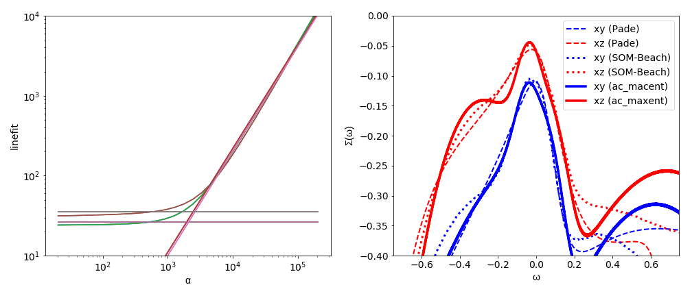
The left graph shows the \(\chi^2\) versus \(\alpha\) curve for all orbitals and spins. Due to the degeneracies we only observe two lines (and their linefits) - one for the xy and one for the xz/yz orbitals - both of them show the characteristic kink.

In the right graph the imaginary part of the resulting self-energies are shown and compared to Padé and the Stochastic Optimization Method (SOM) by Beach [2]. At low energies all methods agree reasonably well. The analysis of the self-energies shows that the xy orbitals are considerably “more incoherent” in Sr₂RuO₄; the self-energy at zero \(\Sigma(\omega = 0)\) is about a factor of \(2\) larger for the xy orbitals.

Footnotes

Continuation of self-energies: Sr2RuO4

Continuation of self-energies: Sr₂RuO₄