Analyzers

This is a list of the implemented analyzers.

class triqs_maxent.analyzers.linefit_analyzer.LineFitAnalyzer(linefit_deg=0, name=None)

Bases: Analyzer

Analyzer searching the kink in \(\chi^2\)

This analyzer fits a piecewise linear function consisting of two straight lines to the function \(\log\chi^2(\log\alpha)\) (the blue curve in the example plot below), using the slope and y-intercept of the linear functions (the orange and green curves in the example plot below) as fit parameters, together with the point where the description changes from one piece to the other. The \(\alpha\)-value closest to their intersection is chosen to give the final spectral function.

import matplotlib.pyplot as plt
import numpy as np
from triqs_maxent.analyzers.linefit_analyzer import fit_piecewise
chi2 = [29349.131935651938, 22046.546280176568, 16571.918154748197, 12487.464413222642, 9445.982385619374, 7178.502063034175, 5481.286491560124, 4203.095677764095, 3233.499702682774, 2492.7723059042005, 1923.6134333677408, 1484.7009011237717, 1145.8924661597946, 884.8005310524965, 684.4330049956029, 531.6146648070567, 415.9506388789646, 329.14872296705806, 264.5685376022979, 216.90786277834727, 181.96883131892676, 156.46999971120204, 137.88618534909426, 124.30790112614721, 114.31767388342703, 106.88286008781692, 101.26499523088836, 96.94522657033058, 93.56467085587808, 90.87798882482437, 88.71820342038981, 86.97077896408142, 85.5551277292544, 84.41192628409034, 83.49484873710317, 82.76553387129734, 82.19079735392212, 81.74128618303814, 81.39095719753091, 81.11694546963328, 80.89956952736446, 80.72238218084304, 80.57227364014592, 80.43956708639224, 80.31784061686754, 80.20324577429295, 80.09354393085312, 79.98731507910087, 79.88352134738581, 79.78132986379869, 79.68005975635513, 79.57917682677997, 79.47830114687353, 79.3772153699245, 79.27587158258149, 79.17439295434937, 79.07307358453718, 78.97237532888748, 78.87292433093153, 78.77550599359282]
alpha = np.logspace(0, np.log10(2.e5) , len(chi2))[::-1]
plt.loglog(alpha, chi2)
plt.xlabel(r'$\alpha$')
plt.ylabel(r'$\chi^2$')
_, p = \
    fit_piecewise(np.log(alpha),
                  np.log(chi2))
yl = plt.ylim()
plt.loglog(alpha, np.exp(p[0][1]+p[0][0]*np.log(alpha)))
plt.loglog(alpha, np.exp(p[1][0]*np.ones(len(alpha))))
plt.ylim(yl)

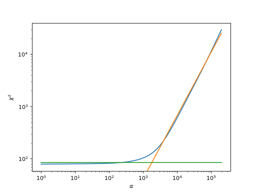
Please be careful to include a sufficient number of \(\alpha\) points; however, when using too large \(\alpha\)-values, the curve starts to flatten again - then, a piecewise fit using three linear curves would be necessary (which is not implemented).

Parameters:

linefit_degint

whether the leftmost piece should have zero slope (linefit_deg=0) or whether its slope should be fitted (linefit_deg=1); defaults to 0.

namestr

the name of the method, defaults to LineFitAnalyzer.

Attributes:

A_outarray (vector)

the output, i.e. the one true spectrum

alpha_indexint

the index of the output in the A_values array

linefit_paramslist

the polyfit parameters of the two lines

infostr

some information about what the analyzer did

Methods

analyze(maxent_result[, matrix_element])

Perform the analysis

analyze(maxent_result, matrix_element=None)

Perform the analysis

Parameters:

maxent_resultMaxEntResult

the result where the \(\alpha\)-dependent data is taken from

matrix_elementtuple

the matrix element (if applicable) that should be analyzed

Returns:

resultAnalyzerResult

the result of the analysis, including the \(A_{out}\)

triqs_maxent.analyzers.linefit_analyzer.fit_piecewise(logx, logy, p2_deg=0)

piecewise linear fit (e.g. for chi2)

The curve is fitted by two linear curves; for the first few indices, the fit is done by choosing both the slope and the y-axis intercept. If p2_deg is 0, a constant curve is fitted (i.e., the only fit parameter is the y-axis intercept) for the last few indices, if it is 1 also the slope is fitted.

The point (i.e., data point index) up to where the first linear curve is used (and from where the second linear curve is used) is also determined by minimizing the misfit. I.e., we search the minimum misfit with respect to the fit parameters of the linear curve and with respect to the index up to where the first curve is used.

Parameters:

logxarray

the x-coordinates of the curve that should be fitted piecewise

logyarray

the y-corrdinates of the curve that should be fitted piecewise

p2_degint

0 or 1, giving the polynomial degree of the second curve

class triqs_maxent.analyzers.chi2_curvature_analyzer.Chi2CurvatureAnalyzer(gamma=0.2, name=None)

Bases: Analyzer

Analyzer using the curvature of \(\chi^2(\alpha)\).

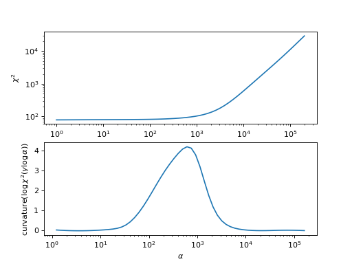
In analogy to the procedure used in the OmegaMaxEnt code, this analyzer chooses the spectral function by searching for the maximum of the curvature of \(\log\chi^2(\gamma \log\alpha)\).

import matplotlib.pyplot as plt
import numpy as np
from triqs_maxent.analyzers.chi2_curvature_analyzer import curv
chi2 = [29349.131935651938, 22046.546280176568, 16571.918154748197, 12487.464413222642, 9445.982385619374, 7178.502063034175, 5481.286491560124, 4203.095677764095, 3233.499702682774, 2492.7723059042005, 1923.6134333677408, 1484.7009011237717, 1145.8924661597946, 884.8005310524965, 684.4330049956029, 531.6146648070567, 415.9506388789646, 329.14872296705806, 264.5685376022979, 216.90786277834727, 181.96883131892676, 156.46999971120204, 137.88618534909426, 124.30790112614721, 114.31767388342703, 106.88286008781692, 101.26499523088836, 96.94522657033058, 93.56467085587808, 90.87798882482437, 88.71820342038981, 86.97077896408142, 85.5551277292544, 84.41192628409034, 83.49484873710317, 82.76553387129734, 82.19079735392212, 81.74128618303814, 81.39095719753091, 81.11694546963328, 80.89956952736446, 80.72238218084304, 80.57227364014592, 80.43956708639224, 80.31784061686754, 80.20324577429295, 80.09354393085312, 79.98731507910087, 79.88352134738581, 79.78132986379869, 79.68005975635513, 79.57917682677997, 79.47830114687353, 79.3772153699245, 79.27587158258149, 79.17439295434937, 79.07307358453718, 78.97237532888748, 78.87292433093153, 78.77550599359282]
alpha = np.logspace(0, np.log10(2.e5) , len(chi2))[::-1]
plt.subplot(2,1,1)
plt.loglog(alpha, chi2)
plt.xlabel(r'$\alpha$')
plt.ylabel(r'$\chi^2$')
plt.subplot(2,1,2)
curv = curv(0.2*np.log10(alpha), np.log10(chi2))[0]
plt.semilogx(alpha, curv)
plt.xlabel(r'$\alpha$')
plt.ylabel(r'$\mathrm{curvature}(\log \chi^2(\gamma \log\alpha))$')

Parameters:

gammafloat

the parameter by which the argument of the curve is multiplied before calculating the curvature, defaults to 0.2

namestr

the name of the method, defaults to Chi2CurvatureAnalyzer.

Attributes:

A_outarray (vector)

the output, i.e. the one true spectrum

alpha_indexint

the index of the output in the A_values array

curvaturearray

the curvature of \(\log\chi^2(\gamma \log\alpha)\)

infostr

some information about what the analyzer did

Methods

analyze(maxent_result[, matrix_element])

Perform the analysis

analyze(maxent_result, matrix_element=None)

Perform the analysis

Parameters:

maxent_resultMaxEntResult

the result where the \(\alpha\)-dependent data is taken from

matrix_elementtuple

the matrix element (if applicable) that should be analyzed

Returns:

resultAnalyzerResult

the result of the analysis, including the \(A_{out}\)

triqs_maxent.analyzers.chi2_curvature_analyzer.curv(x, y)

calculate the curvature of a curve given by x / y data points

The curvature is given by

\[c = \frac{\partial^2 y}{\partial x^2} \Bigg/ \left(1 + \left(\frac{\partial y}{\partial x}\right)^2\right)^{3/2}.\]

The derivatives are calculated using a central finite difference approximation with second-order accuracy. Therefore, the resulting curvature contains nan as first and last entry.

class triqs_maxent.analyzers.entropy_analyzer.EntropyAnalyzer(name=None)

Bases: Analyzer

Analyzer searching a flat feature in the entropy

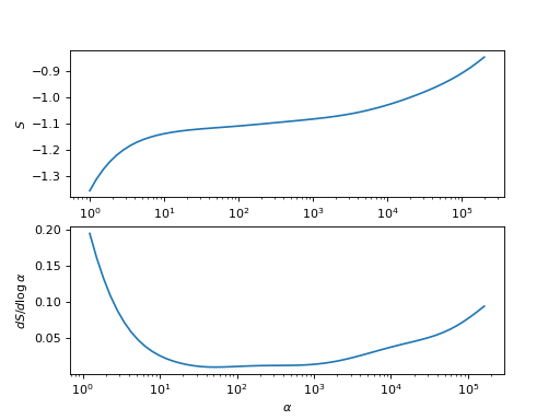
This analyzer chooses the spectrum \(A_\alpha(\omega)\) where the derivative of the entropy with respect to \(\log\alpha\) is minimal.

import matplotlib.pyplot as plt
import numpy as np
S = [-0.8456575058822821, -0.8658403520963711, -0.8844467584579873, -0.9015179804032627, -0.917151672328798, -0.9314863556664439, -0.944683164425082, -0.956907556102252, -0.9683133476777639, -0.9790307680896819, -0.9891593596567183, -0.9987657170111451, -1.0078854019950367, -1.0165280011549969, -1.024684177382945, -1.0323336228063789, -1.0394529560517198, -1.0460227711524488, -1.0520332288852523, -1.057487795325951, -1.062404977107112, -1.0668181517074484, -1.070773798901126, -1.0743285656102701, -1.0775456259846594, -1.08049074893449, -1.0832283965498788, -1.0858180930339953, -1.0883112550281395, -1.0907486650570901, -1.0931587807617578, -1.095557070693374, -1.0979465250594018, -1.1003193968995932, -1.1026600976500056, -1.1049490343932176, -1.1071670792456967, -1.1093003459253266, -1.111345024505977, -1.1133121363430305, -1.1152320138828, -1.1171577437178764, -1.1191656036718212, -1.1213502283233436, -1.1238160022650803, -1.1266718510795215, -1.1300348922182275, -1.1340406305366701, -1.1388547911555023, -1.1446847433171343, -1.1517907169027382, -1.1604971815494127, -1.1712045022410134, -1.1844004970446838, -1.2006707511139032, -1.220706440371579, -1.2453068384914605, -1.2753730596069384, -1.311887106342708, -1.355868667039715]
S = np.array(S)
alpha = np.logspace(0, np.log10(2.e5) , len(S))[::-1]
plt.subplot(2,1,1)
plt.semilogx(alpha, S)
plt.xlabel(r'$\alpha$')
plt.ylabel(r'$S$')
plt.subplot(2,1,2)
deriv = np.full(len(alpha), np.nan)
deriv[1:-1] = ((S[2:] - S[:-2]) / (
    np.log(alpha[2:]) - np.log(alpha[:-2])))
plt.semilogx(alpha, deriv)
plt.xlabel(r'$\alpha$')
plt.ylabel(r'$dS/d\log\alpha$')

Parameters:

namestr

the name of the method, defaults to EntropyAnalyzer.

Attributes:

A_outarray (vector)

the output, i.e. the one true spectrum

alpha_indexint

the index of the output in the A_values array

dS_dalphaarray

the derivative of the entropy with respect to \(\\log\\alpha\)

infostr

some information about what the analyzer did

Methods

analyze(maxent_result[, matrix_element])

Perform the analysis

analyze(maxent_result, matrix_element=None)

Perform the analysis

Parameters:

maxent_resultMaxEntResult

the result where the \(\alpha\)-dependent data is taken from

matrix_elementtuple

the matrix element (if applicable) that should be analyzed

Returns:

resultAnalyzerResult

the result of the analysis, including the \(A_{out}\)

class triqs_maxent.analyzers.classic_analyzer.ClassicAnalyzer(name=None)

Bases: Analyzer

Analyzer using the classic MaxEnt method

This returns the spectrum \(A_\alpha(\omega)\) that has the maximum probability (see BryanAnalyzer for a plot of the probability).

Parameters:

namestr

the name of the method, defaults to ClassicAnalyzer.

Attributes:

A_outarray (vector)

the output, i.e. the one true spectrum

alpha_indexint

the index of the output in the A_values array

infostr

some information about what the analyzer did

Methods

analyze(maxent_result[, matrix_element])

Perform the analysis

analyze(maxent_result, matrix_element=None)

Perform the analysis

Parameters:

maxent_resultMaxEntResult

the result where the \(\alpha\)-dependent data is taken from

matrix_elementtuple

the matrix element (if applicable) that should be analyzed

Returns:

resultAnalyzerResult

the result of the analysis, including the \(A_{out}\)

class triqs_maxent.analyzers.bryan_analyzer.BryanAnalyzer(average_by_integration=False, name=None)

Bases: Analyzer

Bryan’s analyzer

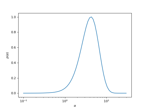
This analyzer averages the spectral \(A_\alpha(\omega)\) over \(\alpha\), weighted by the probability \(p(\alpha)\). This is known as the Bryan MaxEnt method.

Given the probability (e.g., the one in the following plot, which is not normalized), first the correct normalization is performed and then an average over all spectral functions weighted by the probability is done.

The normalized probability is

\[\bar{p} = \sum_i p_i \Delta\alpha_i\]

and the output spectral function is

\[A_{out}(\omega) = \sum_i \bar{p}_i A_{\alpha_i}(\omega) \Delta\alpha_i.\]

If average_by_integration is True, \(\Delta\alpha\) is calculated using the trapezoidal rule; else, it is just taken to be one.

import matplotlib.pyplot as plt
import numpy as np
log_prob = [ -133.77644825014883, -131.1811908969303, -128.87341313304904, -126.82613548679048, -125.01469769984743, -123.41663004550679, -122.01152204906518, -120.78088130473434, -119.70797803270561, -118.77769170465523, -117.9763548787618, -117.29161778070646, -116.71230318712861, -116.22830157384657, -115.83044965526712, -115.51044678567999, -115.26075975426504, -115.07455020581381, -114.94560323182378, -114.86826719005813, -114.83739408789381, -114.84829352389285, -114.89667888116442, -114.97863680101291, -115.0905799690475, -115.22921464699886, -115.39151433606989, -115.5746861915961, -115.77614736900517, -115.99350342514697, -116.2245185175958, -116.4671120942432, -116.71933049377914, -116.97932853127824, -117.24536855479826, -117.5158025086968, -117.78907087999886, -118.06368576040379, -118.33825708524627, -118.61146172746481, -118.88209449357468, -119.14906945217739, -119.41146583894628, -119.66854741331817, -119.91990114496151, -120.16545905975504, -120.4056296141437, -120.64136582811162, -120.87420189716848, -121.10607386134298, -121.3389742988314, -121.57441157558964, -121.81295817443836, -122.05409935782784, -122.29644776767404, -122.53822785898488, -122.77762927908799, -123.01305326403487, -123.24343091919015, -123.46821951105106]
alpha = np.logspace(-1, np.log10(30), len(log_prob))[::-1]
p = np.exp(log_prob - np.max(log_prob))
plt.semilogx(alpha, p)
plt.xlabel(r'$\alpha$')
plt.ylabel(r'$p(\alpha)$')

Parameters:

average_by_integrationbool

if True, the average spectral function is calculated by integrating over all alphas weighted by the probability using the trapezoidal rule; if False (the default), it is calculated by summing over all alphas weighted by the probability

namestr

the name of the method, defaults to BryanAnalyzer.

Attributes:

A_outarray (vector)

the output, i.e. the one true spectrum

infostr

some information about what the analyzer did

Methods

analyze(maxent_result[, matrix_element])

Perform the analysis

analyze(maxent_result, matrix_element=None)

Perform the analysis

Parameters:

maxent_resultMaxEntResult

the result where the \(\alpha\)-dependent data is taken from

matrix_elementtuple

the matrix element (if applicable) that should be analyzed

Returns:

resultAnalyzerResult

the result of the analysis, including the \(A_{out}\)

triqs_maxent.analyzers.bryan_analyzer.get_delta(v)

Get the integration delta for arbitrarily-spaced vector

Parameters:

vnumpy array

values of e.g. omega

Returns:

deltanumpy array

integration delta v for the generalized trapezoidal integration