Fourier and Legendre to Matsubara transforms

Here are the different ways to transform Green’s functions of one type into a different type.

Time to frequency

The command Fourier allows you to initialize a block Green’s function defined in frequency (time) from a block Green’s function defined in time (frequency). Here’s a simple example:

from triqs.gf import *
from triqs.plot.mpl_interface import oplot

# A Green's function on the Matsubara axis set to a semicircular
gw = GfImFreq(indices = [1], beta = 50)
gw << SemiCircular(half_bandwidth = 1)

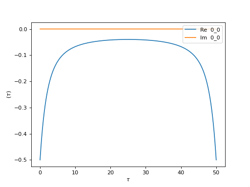
# Create an imaginary-time Green's function and plot it
gt = GfImTime(indices = [1], beta = 50)
gt << Fourier(gw)
oplot(gt, '-')

The same command can be used for real-time <-> real-frequency transformations.

Legendre to Matsubara

The commands MatsubaraToLegendre and LegendreToMatsubara allow to initialize a Matsubara Green’s function (either in imaginary time or in imaginary frequencies) from a Legendre Green’s function and conversely. Example:

from triqs.gf import *
from triqs.plot.mpl_interface import oplot

# A Green's function on the Matsubara axis set to a semicircular
gw = GfImFreq(indices = [1], beta = 50)
gw << SemiCircular(half_bandwidth = 1)

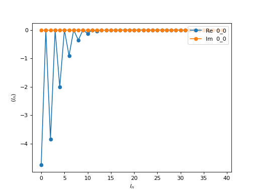
# Create a Legendre Green's function with 40 coefficients
# initialize it from gw and plot it
gl = GfLegendre(indices = [1], beta = 50, n_points = 40)
gl << MatsubaraToLegendre(gw)
oplot(gl, '-o')