Single-orbital Hubbard model
In this notebook you will reproduce the Bethe lattice DMFT that we did earlier with IPT, but you will use the CTHYB solver to find the solution of the impurity problem. We will consider the problem at half-filling again.
In general it is a good idea to develop the script in the notebook, because it is very convenient to find bugs and to quickly come to a working code. In the beginning you should use a small number of Monte Carlo iterations (say 1000) so that the code runs quickly. Your first main goal is to have a functional script. However, once the script is done, we recommend that you do longer runs (production runs) from a shell. It will be easier for you to see the progress of the Monte Carlo solver. Think about saving the relevant data to an archive and then go back to the notebook when it comes to analyzing and plotting the results. This is usually how things are done: elaboration of the scripts and analysis of the data from the notebook, production from a shell.
In order to run your script from a shell, open a terminal and go in the tutorial directory. This is where you should edit your production script. Let’s call it run_dmft.py. Use your favourite editor (e.g. vi or gedit) to create the script run_dmft.py.
When the script is written save it and run it. You can:
run it directly from the shell to see the Monte Carlo progress:
>>> python run_dmft.py
run the following command in a notebook cell.
%run run_dmft.py
That’s it! When the run is done and data has been saved into an archive, you can go back to the notebook and read the archive in order to analyze or plot the results.
Exercise 1
Write a DMFT loop, like you did earlier but using the CTHYB solver.
Hint: It is useful to symmetrize the Green’s function (make the up and down components the same) to avoid some artificial polarization of the system close to the Mott transition. You might want to enforce the up-down symmetry on S.G just before the self-consistency condition. In order to have reasonable data you should have at least 10000 cycles.
Solution 1
The solution of this exercise is in the script scripts/one_band.py in the tutorial directory. We have loaded this script into the cell below.
[1]:
# %load scripts/one_band.py
from triqs.gfs import *
from triqs.operators import *
from h5 import *
from triqs_cthyb import Solver
import numpy as np

# Parameters of the model
t = 1.0
beta = 10
n_loops = 10

# Construct the impurity solver
S = Solver(beta = beta, gf_struct = [('up',1), ('down',1)] )

# I run for several values of U
for U in np.arange(1.0, 9.0):
    print('U =', U)

    # This is a first guess for G
    S.G_iw << SemiCircular(2*t)

    # DMFT loop with self-consistency
    for i in range(n_loops):

        print("\n\nIteration = %i / %i" % (i+1, n_loops))

        # Symmetrize the Green's function and use self-consistency
        g = 0.5 * ( S.G_iw['up'] + S.G_iw['down'] )
        for name, g0 in S.G0_iw:
            g0 << inverse( iOmega_n + U/2.0 - t**2 * g )

        # Solve the impurity problem
        S.solve(h_int = U * n('up',0) * n('down',0),   # Local Hamiltonian
            n_cycles  = 10000,                           # Number of QMC cycles
            n_warmup_cycles = 5000,                      # Warmup cycles
            )

        # Save iteration in archive
        with HDFArchive("data/one_band/half-U%.2f.h5"%U) as A:
            A['G-%i'%i] = S.G_iw
            A['Sigma-%i'%i] = S.Sigma_iw
Warning: could not identify MPI environment!
U = 1.0


Iteration = 1 / 10

╔╦╗╦═╗╦╔═╗ ╔═╗  ┌─┐┌┬┐┬ ┬┬ ┬┌┐
 ║ ╠╦╝║║═╬╗╚═╗  │   │ ├─┤└┬┘├┴┐
 ╩ ╩╚═╩╚═╝╚╚═╝  └─┘ ┴ ┴ ┴ ┴ └─┘

The local Hamiltonian of the problem:
Starting serial run at: 2026-06-28 08:05:34.503668
-0.5*c_dag('down',0)*c('down',0) + -0.5*c_dag('up',0)*c('up',0) + 1*c_dag('down',0)*c_dag('up',0)*c('up',0)*c('down',0)
Using autopartition algorithm to partition the local Hilbert space
Found 4 subspaces.
[Rank 0] Performing warmup phase...
[Rank 0] 08:05:34 22.32% done, ETA 00:00:00, cycle 1116 of 5000, 1.12e+04 cycles/sec
[Rank 0] 08:05:35 100.00% done, ETA 00:00:00, cycle 5000 of 5000, 1.14e+04 cycles/sec
[Rank 0] Performing accumulation phase...
[Rank 0] 08:05:35 11.38% done, ETA 00:00:00, cycle 1138 of 10000, 1.14e+04 cycles/sec
[Rank 0] 08:05:35 100.00% done, ETA 00:00:00, cycle 10000 of 10000, 1.13e+04 cycles/sec
[Rank 0] Collect results: Waiting for all MPI processes to finish accumulating...
[Rank 0] Warmup duration: 0.4401 seconds [00:00:00]
[Rank 0] Simulation duration: 0.8815 seconds [00:00:00]
[Rank 0] Number of measures: 10000
[Rank 0] Cycles (measures) / second: 1.13e+04
[Rank 0] Measurement durations (total = 0.0048):
[Rank 0] Measure Auto-correlation time: Duration = 0.0010
[Rank 0] Measure Average order: Duration = 0.0002
[Rank 0] Measure Average sign: Duration = 0.0002
[Rank 0] Measure G_tau measure: Duration = 0.0033
[Rank 0] Move durations (total = 0.8472):
[Rank 0] Move set Insert two operators: Duration = 0.1271
[Rank 0] Move Insert Delta_up: Duration = 0.0591
[Rank 0] Move Insert Delta_down: Duration = 0.0595
[Rank 0] Move set Remove two operators: Duration = 0.1193
[Rank 0] Move Remove Delta_up: Duration = 0.0554
[Rank 0] Move Remove Delta_down: Duration = 0.0553
[Rank 0] Move set Insert four operators: Duration = 0.1569
[Rank 0] Move Insert Delta_up_up: Duration = 0.0418
[Rank 0] Move Insert Delta_up_down: Duration = 0.0320
[Rank 0] Move Insert Delta_down_up: Duration = 0.0318
[Rank 0] Move Insert Delta_down_down: Duration = 0.0421
[Rank 0] Move set Remove four operators: Duration = 0.1045
[Rank 0] Move Remove Delta_up_up: Duration = 0.0199
[Rank 0] Move Remove Delta_up_down: Duration = 0.0274
[Rank 0] Move Remove Delta_down_up: Duration = 0.0273
[Rank 0] Move Remove Delta_down_down: Duration = 0.0205
[Rank 0] Move Shift one operator: Duration = 0.3393
[Rank 0] Move statistics:
[Rank 0] Move set Insert two operators: Proposed = 100057, Accepted = 13427, Rate = 0.1342
[Rank 0] Move Insert Delta_up: Proposed = 49868, Accepted = 6739, Rate = 0.1351
[Rank 0] Move Insert Delta_down: Proposed = 50189, Accepted = 6688, Rate = 0.1333
[Rank 0] Move set Remove two operators: Proposed = 99733, Accepted = 13372, Rate = 0.1341
[Rank 0] Move Remove Delta_up: Proposed = 49920, Accepted = 6714, Rate = 0.1345
[Rank 0] Move Remove Delta_down: Proposed = 49813, Accepted = 6658, Rate = 0.1337
[Rank 0] Move set Insert four operators: Proposed = 100124, Accepted = 2375, Rate = 0.0237
[Rank 0] Move Insert Delta_up_up: Proposed = 25131, Accepted = 663, Rate = 0.0264
[Rank 0] Move Insert Delta_up_down: Proposed = 24969, Accepted = 537, Rate = 0.0215
[Rank 0] Move Insert Delta_down_up: Proposed = 24998, Accepted = 482, Rate = 0.0193
[Rank 0] Move Insert Delta_down_down: Proposed = 25026, Accepted = 693, Rate = 0.0277
[Rank 0] Move set Remove four operators: Proposed = 99739, Accepted = 2401, Rate = 0.0241
[Rank 0] Move Remove Delta_up_up: Proposed = 24728, Accepted = 675, Rate = 0.0273
[Rank 0] Move Remove Delta_up_down: Proposed = 25161, Accepted = 506, Rate = 0.0201
[Rank 0] Move Remove Delta_down_up: Proposed = 24828, Accepted = 513, Rate = 0.0207
[Rank 0] Move Remove Delta_down_down: Proposed = 25022, Accepted = 707, Rate = 0.0283
[Rank 0] Move Shift one operator: Proposed = 100347, Accepted = 84155, Rate = 0.8386
Total number of measures: 10000
Total cycles (measures) / second: 1.13e+04
Average sign: 1
Average order: 8.1807
Auto-correlation time: 1.58633 cycles
Iteration = 2 / 10
╔╦╗╦═╗╦╔═╗ ╔═╗ ┌─┐┌┬┐┬ ┬┬ ┬┌┐
║ ╠╦╝║║═╬╗╚═╗ │ │ ├─┤└┬┘├┴┐
╩ ╩╚═╩╚═╝╚╚═╝ └─┘ ┴ ┴ ┴ ┴ └─┘
The local Hamiltonian of the problem:
-0.5*c_dag('down',0)*c('down',0) + -0.5*c_dag('up',0)*c('up',0) + 1*c_dag('down',0)*c_dag('up',0)*c('up',0)*c('down',0)
Using autopartition algorithm to partition the local Hilbert space
Found 4 subspaces.
[Rank 0] Performing warmup phase...
[Rank 0] 08:05:36 22.86% done, ETA 00:00:00, cycle 1143 of 5000, 1.14e+04 cycles/sec
[Rank 0] 08:05:36 100.00% done, ETA 00:00:00, cycle 5000 of 5000, 1.13e+04 cycles/sec
[Rank 0] Performing accumulation phase...
[Rank 0] 08:05:36 11.23% done, ETA 00:00:00, cycle 1123 of 10000, 1.12e+04 cycles/sec
[Rank 0] 08:05:37 100.00% done, ETA 00:00:00, cycle 10000 of 10000, 1.11e+04 cycles/sec
[Rank 0] Collect results: Waiting for all MPI processes to finish accumulating...
[Rank 0] Warmup duration: 0.4412 seconds [00:00:00]
[Rank 0] Simulation duration: 0.8993 seconds [00:00:00]
[Rank 0] Number of measures: 10000
[Rank 0] Cycles (measures) / second: 1.11e+04
[Rank 0] Measurement durations (total = 0.0050):
[Rank 0] Measure Auto-correlation time: Duration = 0.0011
[Rank 0] Measure Average order: Duration = 0.0003
[Rank 0] Measure Average sign: Duration = 0.0002
[Rank 0] Measure G_tau measure: Duration = 0.0034
[Rank 0] Move durations (total = 0.8639):
[Rank 0] Move set Insert two operators: Duration = 0.1308
[Rank 0] Move Insert Delta_up: Duration = 0.0610
[Rank 0] Move Insert Delta_down: Duration = 0.0609
[Rank 0] Move set Remove two operators: Duration = 0.1222
[Rank 0] Move Remove Delta_up: Duration = 0.0570
[Rank 0] Move Remove Delta_down: Duration = 0.0563
[Rank 0] Move set Insert four operators: Duration = 0.1604
[Rank 0] Move Insert Delta_up_up: Duration = 0.0431
[Rank 0] Move Insert Delta_up_down: Duration = 0.0324
[Rank 0] Move Insert Delta_down_up: Duration = 0.0326
[Rank 0] Move Insert Delta_down_down: Duration = 0.0429
[Rank 0] Move set Remove four operators: Duration = 0.1069
[Rank 0] Move Remove Delta_up_up: Duration = 0.0206
[Rank 0] Move Remove Delta_up_down: Duration = 0.0280
[Rank 0] Move Remove Delta_down_up: Duration = 0.0279
[Rank 0] Move Remove Delta_down_down: Duration = 0.0211
[Rank 0] Move Shift one operator: Duration = 0.3434
[Rank 0] Move statistics:
[Rank 0] Move set Insert two operators: Proposed = 99935, Accepted = 13744, Rate = 0.1375
[Rank 0] Move Insert Delta_up: Proposed = 49896, Accepted = 6916, Rate = 0.1386
[Rank 0] Move Insert Delta_down: Proposed = 50039, Accepted = 6828, Rate = 0.1365
[Rank 0] Move set Remove two operators: Proposed = 99870, Accepted = 13547, Rate = 0.1356
[Rank 0] Move Remove Delta_up: Proposed = 50031, Accepted = 6859, Rate = 0.1371
[Rank 0] Move Remove Delta_down: Proposed = 49839, Accepted = 6688, Rate = 0.1342
[Rank 0] Move set Insert four operators: Proposed = 100015, Accepted = 2481, Rate = 0.0248
[Rank 0] Move Insert Delta_up_up: Proposed = 25118, Accepted = 729, Rate = 0.0290
[Rank 0] Move Insert Delta_up_down: Proposed = 24879, Accepted = 505, Rate = 0.0203
[Rank 0] Move Insert Delta_down_up: Proposed = 24988, Accepted = 530, Rate = 0.0212
[Rank 0] Move Insert Delta_down_down: Proposed = 25030, Accepted = 717, Rate = 0.0286
[Rank 0] Move set Remove four operators: Proposed = 99804, Accepted = 2576, Rate = 0.0258
[Rank 0] Move Remove Delta_up_up: Proposed = 24789, Accepted = 744, Rate = 0.0300
[Rank 0] Move Remove Delta_up_down: Proposed = 25153, Accepted = 523, Rate = 0.0208
[Rank 0] Move Remove Delta_down_up: Proposed = 24858, Accepted = 537, Rate = 0.0216
[Rank 0] Move Remove Delta_down_down: Proposed = 25004, Accepted = 772, Rate = 0.0309
[Rank 0] Move Shift one operator: Proposed = 100376, Accepted = 83279, Rate = 0.8297
Total number of measures: 10000
Total cycles (measures) / second: 1.11e+04
Average sign: 1
Average order: 8.0726
Auto-correlation time: 1.71842 cycles
Iteration = 3 / 10
╔╦╗╦═╗╦╔═╗ ╔═╗ ┌─┐┌┬┐┬ ┬┬ ┬┌┐
║ ╠╦╝║║═╬╗╚═╗ │ │ ├─┤└┬┘├┴┐
╩ ╩╚═╩╚═╝╚╚═╝ └─┘ ┴ ┴ ┴ ┴ └─┘
The local Hamiltonian of the problem:
-0.5*c_dag('down',0)*c('down',0) + -0.5*c_dag('up',0)*c('up',0) + 1*c_dag('down',0)*c_dag('up',0)*c('up',0)*c('down',0)
Using autopartition algorithm to partition the local Hilbert space
Found 4 subspaces.
[Rank 0] Performing warmup phase...
[Rank 0] 08:05:37 21.76% done, ETA 00:00:00, cycle 1088 of 5000, 1.09e+04 cycles/sec
[Rank 0] 08:05:37 100.00% done, ETA 00:00:00, cycle 5000 of 5000, 1.15e+04 cycles/sec
[Rank 0] Performing accumulation phase...
[Rank 0] 08:05:37 12.73% done, ETA 00:00:00, cycle 1273 of 10000, 1.27e+04 cycles/sec
[Rank 0] 08:05:38 100.00% done, ETA 00:00:00, cycle 10000 of 10000, 1.17e+04 cycles/sec
[Rank 0] Collect results: Waiting for all MPI processes to finish accumulating...
[Rank 0] Warmup duration: 0.4360 seconds [00:00:00]
[Rank 0] Simulation duration: 0.8567 seconds [00:00:00]
[Rank 0] Number of measures: 10000
[Rank 0] Cycles (measures) / second: 1.17e+04
[Rank 0] Measurement durations (total = 0.0047):
[Rank 0] Measure Auto-correlation time: Duration = 0.0011
[Rank 0] Measure Average order: Duration = 0.0002
[Rank 0] Measure Average sign: Duration = 0.0003
[Rank 0] Measure G_tau measure: Duration = 0.0031
[Rank 0] Move durations (total = 0.8238):
[Rank 0] Move set Insert two operators: Duration = 0.1246
[Rank 0] Move Insert Delta_up: Duration = 0.0577
[Rank 0] Move Insert Delta_down: Duration = 0.0584
[Rank 0] Move set Remove two operators: Duration = 0.1164
[Rank 0] Move Remove Delta_up: Duration = 0.0537
[Rank 0] Move Remove Delta_down: Duration = 0.0542
[Rank 0] Move set Insert four operators: Duration = 0.1527
[Rank 0] Move Insert Delta_up_up: Duration = 0.0408
[Rank 0] Move Insert Delta_up_down: Duration = 0.0309
[Rank 0] Move Insert Delta_down_up: Duration = 0.0310
[Rank 0] Move Insert Delta_down_down: Duration = 0.0409
[Rank 0] Move set Remove four operators: Duration = 0.1015
[Rank 0] Move Remove Delta_up_up: Duration = 0.0199
[Rank 0] Move Remove Delta_up_down: Duration = 0.0266
[Rank 0] Move Remove Delta_down_up: Duration = 0.0265
[Rank 0] Move Remove Delta_down_down: Duration = 0.0197
[Rank 0] Move Shift one operator: Duration = 0.3286
[Rank 0] Move statistics:
[Rank 0] Move set Insert two operators: Proposed = 100109, Accepted = 13684, Rate = 0.1367
[Rank 0] Move Insert Delta_up: Proposed = 49942, Accepted = 6798, Rate = 0.1361
[Rank 0] Move Insert Delta_down: Proposed = 50167, Accepted = 6886, Rate = 0.1373
[Rank 0] Move set Remove two operators: Proposed = 99700, Accepted = 13554, Rate = 0.1359
[Rank 0] Move Remove Delta_up: Proposed = 49876, Accepted = 6739, Rate = 0.1351
[Rank 0] Move Remove Delta_down: Proposed = 49824, Accepted = 6815, Rate = 0.1368
[Rank 0] Move set Insert four operators: Proposed = 99996, Accepted = 2443, Rate = 0.0244
[Rank 0] Move Insert Delta_up_up: Proposed = 25032, Accepted = 700, Rate = 0.0280
[Rank 0] Move Insert Delta_up_down: Proposed = 24885, Accepted = 529, Rate = 0.0213
[Rank 0] Move Insert Delta_down_up: Proposed = 24986, Accepted = 534, Rate = 0.0214
[Rank 0] Move Insert Delta_down_down: Proposed = 25093, Accepted = 680, Rate = 0.0271
[Rank 0] Move set Remove four operators: Proposed = 99732, Accepted = 2507, Rate = 0.0251
[Rank 0] Move Remove Delta_up_up: Proposed = 24863, Accepted = 743, Rate = 0.0299
[Rank 0] Move Remove Delta_up_down: Proposed = 25007, Accepted = 513, Rate = 0.0205
[Rank 0] Move Remove Delta_down_up: Proposed = 24875, Accepted = 522, Rate = 0.0210
[Rank 0] Move Remove Delta_down_down: Proposed = 24987, Accepted = 729, Rate = 0.0292
[Rank 0] Move Shift one operator: Proposed = 100463, Accepted = 83671, Rate = 0.8329
Total number of measures: 10000
Total cycles (measures) / second: 1.17e+04
Average sign: 1
Average order: 8.1617
Auto-correlation time: 1.43877 cycles
Iteration = 4 / 10
╔╦╗╦═╗╦╔═╗ ╔═╗ ┌─┐┌┬┐┬ ┬┬ ┬┌┐
║ ╠╦╝║║═╬╗╚═╗ │ │ ├─┤└┬┘├┴┐
╩ ╩╚═╩╚═╝╚╚═╝ └─┘ ┴ ┴ ┴ ┴ └─┘
The local Hamiltonian of the problem:
-0.5*c_dag('down',0)*c('down',0) + -0.5*c_dag('up',0)*c('up',0) + 1*c_dag('down',0)*c_dag('up',0)*c('up',0)*c('down',0)
Using autopartition algorithm to partition the local Hilbert space
Found 4 subspaces.
[Rank 0] Performing warmup phase...
[Rank 0] 08:05:38 22.10% done, ETA 00:00:00, cycle 1105 of 5000, 1.10e+04 cycles/sec
[Rank 0] 08:05:39 100.00% done, ETA 00:00:00, cycle 5000 of 5000, 1.11e+04 cycles/sec
[Rank 0] Performing accumulation phase...
[Rank 0] 08:05:39 11.09% done, ETA 00:00:00, cycle 1109 of 10000, 1.11e+04 cycles/sec
[Rank 0] 08:05:40 100.00% done, ETA 00:00:00, cycle 10000 of 10000, 1.16e+04 cycles/sec
[Rank 0] Collect results: Waiting for all MPI processes to finish accumulating...
[Rank 0] Warmup duration: 0.4505 seconds [00:00:00]
[Rank 0] Simulation duration: 0.8602 seconds [00:00:00]
[Rank 0] Number of measures: 10000
[Rank 0] Cycles (measures) / second: 1.16e+04
[Rank 0] Measurement durations (total = 0.0045):
[Rank 0] Measure Auto-correlation time: Duration = 0.0010
[Rank 0] Measure Average order: Duration = 0.0003
[Rank 0] Measure Average sign: Duration = 0.0002
[Rank 0] Measure G_tau measure: Duration = 0.0030
[Rank 0] Move durations (total = 0.8267):
[Rank 0] Move set Insert two operators: Duration = 0.1255
[Rank 0] Move Insert Delta_up: Duration = 0.0585
[Rank 0] Move Insert Delta_down: Duration = 0.0585
[Rank 0] Move set Remove two operators: Duration = 0.1174
[Rank 0] Move Remove Delta_up: Duration = 0.0544
[Rank 0] Move Remove Delta_down: Duration = 0.0544
[Rank 0] Move set Insert four operators: Duration = 0.1526
[Rank 0] Move Insert Delta_up_up: Duration = 0.0409
[Rank 0] Move Insert Delta_up_down: Duration = 0.0308
[Rank 0] Move Insert Delta_down_up: Duration = 0.0309
[Rank 0] Move Insert Delta_down_down: Duration = 0.0410
[Rank 0] Move set Remove four operators: Duration = 0.1017
[Rank 0] Move Remove Delta_up_up: Duration = 0.0195
[Rank 0] Move Remove Delta_up_down: Duration = 0.0270
[Rank 0] Move Remove Delta_down_up: Duration = 0.0266
[Rank 0] Move Remove Delta_down_down: Duration = 0.0197
[Rank 0] Move Shift one operator: Duration = 0.3296
[Rank 0] Move statistics:
[Rank 0] Move set Insert two operators: Proposed = 100024, Accepted = 13791, Rate = 0.1379
[Rank 0] Move Insert Delta_up: Proposed = 49964, Accepted = 6934, Rate = 0.1388
[Rank 0] Move Insert Delta_down: Proposed = 50060, Accepted = 6857, Rate = 0.1370
[Rank 0] Move set Remove two operators: Proposed = 99738, Accepted = 13650, Rate = 0.1369
[Rank 0] Move Remove Delta_up: Proposed = 49897, Accepted = 6878, Rate = 0.1378
[Rank 0] Move Remove Delta_down: Proposed = 49841, Accepted = 6772, Rate = 0.1359
[Rank 0] Move set Insert four operators: Proposed = 99833, Accepted = 2400, Rate = 0.0240
[Rank 0] Move Insert Delta_up_up: Proposed = 25012, Accepted = 699, Rate = 0.0279
[Rank 0] Move Insert Delta_up_down: Proposed = 24901, Accepted = 481, Rate = 0.0193
[Rank 0] Move Insert Delta_down_up: Proposed = 24940, Accepted = 512, Rate = 0.0205
[Rank 0] Move Insert Delta_down_down: Proposed = 24980, Accepted = 708, Rate = 0.0283
[Rank 0] Move set Remove four operators: Proposed = 99991, Accepted = 2472, Rate = 0.0247
[Rank 0] Move Remove Delta_up_up: Proposed = 24883, Accepted = 677, Rate = 0.0272
[Rank 0] Move Remove Delta_up_down: Proposed = 25159, Accepted = 553, Rate = 0.0220
[Rank 0] Move Remove Delta_down_up: Proposed = 24828, Accepted = 542, Rate = 0.0218
[Rank 0] Move Remove Delta_down_down: Proposed = 25121, Accepted = 700, Rate = 0.0279
[Rank 0] Move Shift one operator: Proposed = 100414, Accepted = 83376, Rate = 0.8303
Total number of measures: 10000
Total cycles (measures) / second: 1.16e+04
Average sign: 1
Average order: 8.1484
Auto-correlation time: 1.56079 cycles
Iteration = 5 / 10
╔╦╗╦═╗╦╔═╗ ╔═╗ ┌─┐┌┬┐┬ ┬┬ ┬┌┐
║ ╠╦╝║║═╬╗╚═╗ │ │ ├─┤└┬┘├┴┐
╩ ╩╚═╩╚═╝╚╚═╝ └─┘ ┴ ┴ ┴ ┴ └─┘
The local Hamiltonian of the problem:
-0.5*c_dag('down',0)*c('down',0) + -0.5*c_dag('up',0)*c('up',0) + 1*c_dag('down',0)*c_dag('up',0)*c('up',0)*c('down',0)
Using autopartition algorithm to partition the local Hilbert space
Found 4 subspaces.
[Rank 0] Performing warmup phase...
[Rank 0] 08:05:40 24.04% done, ETA 00:00:00, cycle 1202 of 5000, 1.20e+04 cycles/sec
[Rank 0] 08:05:40 100.00% done, ETA 00:00:00, cycle 5000 of 5000, 1.23e+04 cycles/sec
[Rank 0] Performing accumulation phase...
[Rank 0] 08:05:40 12.20% done, ETA 00:00:00, cycle 1220 of 10000, 1.22e+04 cycles/sec
[Rank 0] 08:05:41 100.00% done, ETA 00:00:00, cycle 10000 of 10000, 1.18e+04 cycles/sec
[Rank 0] Collect results: Waiting for all MPI processes to finish accumulating...
[Rank 0] Warmup duration: 0.4071 seconds [00:00:00]
[Rank 0] Simulation duration: 0.8456 seconds [00:00:00]
[Rank 0] Number of measures: 10000
[Rank 0] Cycles (measures) / second: 1.18e+04
[Rank 0] Measurement durations (total = 0.0044):
[Rank 0] Measure Auto-correlation time: Duration = 0.0010
[Rank 0] Measure Average order: Duration = 0.0002
[Rank 0] Measure Average sign: Duration = 0.0002
[Rank 0] Measure G_tau measure: Duration = 0.0030
[Rank 0] Move durations (total = 0.8128):
[Rank 0] Move set Insert two operators: Duration = 0.1225
[Rank 0] Move Insert Delta_up: Duration = 0.0567
[Rank 0] Move Insert Delta_down: Duration = 0.0573
[Rank 0] Move set Remove two operators: Duration = 0.1159
[Rank 0] Move Remove Delta_up: Duration = 0.0535
[Rank 0] Move Remove Delta_down: Duration = 0.0538
[Rank 0] Move set Insert four operators: Duration = 0.1505
[Rank 0] Move Insert Delta_up_up: Duration = 0.0403
[Rank 0] Move Insert Delta_up_down: Duration = 0.0304
[Rank 0] Move Insert Delta_down_up: Duration = 0.0306
[Rank 0] Move Insert Delta_down_down: Duration = 0.0402
[Rank 0] Move set Remove four operators: Duration = 0.1001
[Rank 0] Move Remove Delta_up_up: Duration = 0.0190
[Rank 0] Move Remove Delta_up_down: Duration = 0.0266
[Rank 0] Move Remove Delta_down_up: Duration = 0.0260
[Rank 0] Move Remove Delta_down_down: Duration = 0.0194
[Rank 0] Move Shift one operator: Duration = 0.3238
[Rank 0] Move statistics:
[Rank 0] Move set Insert two operators: Proposed = 99964, Accepted = 13608, Rate = 0.1361
[Rank 0] Move Insert Delta_up: Proposed = 49895, Accepted = 6751, Rate = 0.1353
[Rank 0] Move Insert Delta_down: Proposed = 50069, Accepted = 6857, Rate = 0.1370
[Rank 0] Move set Remove two operators: Proposed = 99798, Accepted = 13685, Rate = 0.1371
[Rank 0] Move Remove Delta_up: Proposed = 49934, Accepted = 6826, Rate = 0.1367
[Rank 0] Move Remove Delta_down: Proposed = 49864, Accepted = 6859, Rate = 0.1376
[Rank 0] Move set Insert four operators: Proposed = 99996, Accepted = 2460, Rate = 0.0246
[Rank 0] Move Insert Delta_up_up: Proposed = 25113, Accepted = 708, Rate = 0.0282
[Rank 0] Move Insert Delta_up_down: Proposed = 24875, Accepted = 517, Rate = 0.0208
[Rank 0] Move Insert Delta_down_up: Proposed = 24943, Accepted = 541, Rate = 0.0217
[Rank 0] Move Insert Delta_down_down: Proposed = 25065, Accepted = 694, Rate = 0.0277
[Rank 0] Move set Remove four operators: Proposed = 99809, Accepted = 2421, Rate = 0.0243
[Rank 0] Move Remove Delta_up_up: Proposed = 24788, Accepted = 674, Rate = 0.0272
[Rank 0] Move Remove Delta_up_down: Proposed = 25220, Accepted = 545, Rate = 0.0216
[Rank 0] Move Remove Delta_down_up: Proposed = 24797, Accepted = 503, Rate = 0.0203
[Rank 0] Move Remove Delta_down_down: Proposed = 25004, Accepted = 699, Rate = 0.0280
[Rank 0] Move Shift one operator: Proposed = 100433, Accepted = 83401, Rate = 0.8304
Total number of measures: 10000
Total cycles (measures) / second: 1.18e+04
Average sign: 1
Average order: 8.1626
Auto-correlation time: 1.81841 cycles
Iteration = 6 / 10
╔╦╗╦═╗╦╔═╗ ╔═╗ ┌─┐┌┬┐┬ ┬┬ ┬┌┐
║ ╠╦╝║║═╬╗╚═╗ │ │ ├─┤└┬┘├┴┐
╩ ╩╚═╩╚═╝╚╚═╝ └─┘ ┴ ┴ ┴ ┴ └─┘
The local Hamiltonian of the problem:
-0.5*c_dag('down',0)*c('down',0) + -0.5*c_dag('up',0)*c('up',0) + 1*c_dag('down',0)*c_dag('up',0)*c('up',0)*c('down',0)
Using autopartition algorithm to partition the local Hilbert space
Found 4 subspaces.
[Rank 0] Performing warmup phase...
[Rank 0] 08:05:41 24.62% done, ETA 00:00:00, cycle 1231 of 5000, 1.23e+04 cycles/sec
[Rank 0] 08:05:41 100.00% done, ETA 00:00:00, cycle 5000 of 5000, 1.23e+04 cycles/sec
[Rank 0] Performing accumulation phase...
[Rank 0] 08:05:41 12.19% done, ETA 00:00:00, cycle 1219 of 10000, 1.22e+04 cycles/sec
[Rank 0] 08:05:42 100.00% done, ETA 00:00:00, cycle 10000 of 10000, 1.23e+04 cycles/sec
[Rank 0] Collect results: Waiting for all MPI processes to finish accumulating...
[Rank 0] Warmup duration: 0.4074 seconds [00:00:00]
[Rank 0] Simulation duration: 0.8100 seconds [00:00:00]
[Rank 0] Number of measures: 10000
[Rank 0] Cycles (measures) / second: 1.23e+04
[Rank 0] Measurement durations (total = 0.0043):
[Rank 0] Measure Auto-correlation time: Duration = 0.0010
[Rank 0] Measure Average order: Duration = 0.0002
[Rank 0] Measure Average sign: Duration = 0.0002
[Rank 0] Measure G_tau measure: Duration = 0.0028
[Rank 0] Move durations (total = 0.7789):
[Rank 0] Move set Insert two operators: Duration = 0.1175
[Rank 0] Move Insert Delta_up: Duration = 0.0547
[Rank 0] Move Insert Delta_down: Duration = 0.0547
[Rank 0] Move set Remove two operators: Duration = 0.1113
[Rank 0] Move Remove Delta_up: Duration = 0.0518
[Rank 0] Move Remove Delta_down: Duration = 0.0514
[Rank 0] Move set Insert four operators: Duration = 0.1443
[Rank 0] Move Insert Delta_up_up: Duration = 0.0387
[Rank 0] Move Insert Delta_up_down: Duration = 0.0291
[Rank 0] Move Insert Delta_down_up: Duration = 0.0292
[Rank 0] Move Insert Delta_down_down: Duration = 0.0388
[Rank 0] Move set Remove four operators: Duration = 0.0962
[Rank 0] Move Remove Delta_up_up: Duration = 0.0187
[Rank 0] Move Remove Delta_up_down: Duration = 0.0254
[Rank 0] Move Remove Delta_down_up: Duration = 0.0250
[Rank 0] Move Remove Delta_down_down: Duration = 0.0188
[Rank 0] Move Shift one operator: Duration = 0.3097
[Rank 0] Move statistics:
[Rank 0] Move set Insert two operators: Proposed = 99816, Accepted = 13638, Rate = 0.1366
[Rank 0] Move Insert Delta_up: Proposed = 49836, Accepted = 6875, Rate = 0.1380
[Rank 0] Move Insert Delta_down: Proposed = 49980, Accepted = 6763, Rate = 0.1353
[Rank 0] Move set Remove two operators: Proposed = 99894, Accepted = 13796, Rate = 0.1381
[Rank 0] Move Remove Delta_up: Proposed = 50036, Accepted = 6923, Rate = 0.1384
[Rank 0] Move Remove Delta_down: Proposed = 49858, Accepted = 6873, Rate = 0.1379
[Rank 0] Move set Insert four operators: Proposed = 99994, Accepted = 2571, Rate = 0.0257
[Rank 0] Move Insert Delta_up_up: Proposed = 25109, Accepted = 737, Rate = 0.0294
[Rank 0] Move Insert Delta_up_down: Proposed = 24911, Accepted = 530, Rate = 0.0213
[Rank 0] Move Insert Delta_down_up: Proposed = 25010, Accepted = 541, Rate = 0.0216
[Rank 0] Move Insert Delta_down_down: Proposed = 24964, Accepted = 763, Rate = 0.0306
[Rank 0] Move set Remove four operators: Proposed = 99927, Accepted = 2493, Rate = 0.0249
[Rank 0] Move Remove Delta_up_up: Proposed = 24807, Accepted = 721, Rate = 0.0291
[Rank 0] Move Remove Delta_up_down: Proposed = 25231, Accepted = 540, Rate = 0.0214
[Rank 0] Move Remove Delta_down_up: Proposed = 24879, Accepted = 517, Rate = 0.0208
[Rank 0] Move Remove Delta_down_down: Proposed = 25010, Accepted = 715, Rate = 0.0286
[Rank 0] Move Shift one operator: Proposed = 100369, Accepted = 83328, Rate = 0.8302
Total number of measures: 10000
Total cycles (measures) / second: 1.23e+04
Average sign: 1
Average order: 8.1595
Auto-correlation time: 1.96462 cycles
Iteration = 7 / 10
╔╦╗╦═╗╦╔═╗ ╔═╗ ┌─┐┌┬┐┬ ┬┬ ┬┌┐
║ ╠╦╝║║═╬╗╚═╗ │ │ ├─┤└┬┘├┴┐
╩ ╩╚═╩╚═╝╚╚═╝ └─┘ ┴ ┴ ┴ ┴ └─┘
The local Hamiltonian of the problem:
-0.5*c_dag('down',0)*c('down',0) + -0.5*c_dag('up',0)*c('up',0) + 1*c_dag('down',0)*c_dag('up',0)*c('up',0)*c('down',0)
Using autopartition algorithm to partition the local Hilbert space
Found 4 subspaces.
[Rank 0] Performing warmup phase...
[Rank 0] 08:05:42 22.72% done, ETA 00:00:00, cycle 1136 of 5000, 1.14e+04 cycles/sec
[Rank 0] 08:05:43 100.00% done, ETA 00:00:00, cycle 5000 of 5000, 1.21e+04 cycles/sec
[Rank 0] Performing accumulation phase...
[Rank 0] 08:05:43 13.61% done, ETA 00:00:00, cycle 1361 of 10000, 1.36e+04 cycles/sec
[Rank 0] 08:05:43 100.00% done, ETA 00:00:00, cycle 10000 of 10000, 1.25e+04 cycles/sec
[Rank 0] Collect results: Waiting for all MPI processes to finish accumulating...
[Rank 0] Warmup duration: 0.4146 seconds [00:00:00]
[Rank 0] Simulation duration: 0.8008 seconds [00:00:00]
[Rank 0] Number of measures: 10000
[Rank 0] Cycles (measures) / second: 1.25e+04
[Rank 0] Measurement durations (total = 0.0041):
[Rank 0] Measure Auto-correlation time: Duration = 0.0009
[Rank 0] Measure Average order: Duration = 0.0002
[Rank 0] Measure Average sign: Duration = 0.0002
[Rank 0] Measure G_tau measure: Duration = 0.0027
[Rank 0] Move durations (total = 0.7700):
[Rank 0] Move set Insert two operators: Duration = 0.1173
[Rank 0] Move Insert Delta_up: Duration = 0.0544
[Rank 0] Move Insert Delta_down: Duration = 0.0549
[Rank 0] Move set Remove two operators: Duration = 0.1092
[Rank 0] Move Remove Delta_up: Duration = 0.0506
[Rank 0] Move Remove Delta_down: Duration = 0.0507
[Rank 0] Move set Insert four operators: Duration = 0.1421
[Rank 0] Move Insert Delta_up_up: Duration = 0.0381
[Rank 0] Move Insert Delta_up_down: Duration = 0.0287
[Rank 0] Move Insert Delta_down_up: Duration = 0.0289
[Rank 0] Move Insert Delta_down_down: Duration = 0.0380
[Rank 0] Move set Remove four operators: Duration = 0.0949
[Rank 0] Move Remove Delta_up_up: Duration = 0.0181
[Rank 0] Move Remove Delta_up_down: Duration = 0.0252
[Rank 0] Move Remove Delta_down_up: Duration = 0.0252
[Rank 0] Move Remove Delta_down_down: Duration = 0.0182
[Rank 0] Move Shift one operator: Duration = 0.3065
[Rank 0] Move statistics:
[Rank 0] Move set Insert two operators: Proposed = 100041, Accepted = 13874, Rate = 0.1387
[Rank 0] Move Insert Delta_up: Proposed = 49926, Accepted = 6929, Rate = 0.1388
[Rank 0] Move Insert Delta_down: Proposed = 50115, Accepted = 6945, Rate = 0.1386
[Rank 0] Move set Remove two operators: Proposed = 99689, Accepted = 13507, Rate = 0.1355
[Rank 0] Move Remove Delta_up: Proposed = 49950, Accepted = 6735, Rate = 0.1348
[Rank 0] Move Remove Delta_down: Proposed = 49739, Accepted = 6772, Rate = 0.1362
[Rank 0] Move set Insert four operators: Proposed = 99817, Accepted = 2384, Rate = 0.0239
[Rank 0] Move Insert Delta_up_up: Proposed = 25089, Accepted = 708, Rate = 0.0282
[Rank 0] Move Insert Delta_up_down: Proposed = 24883, Accepted = 467, Rate = 0.0188
[Rank 0] Move Insert Delta_down_up: Proposed = 24887, Accepted = 531, Rate = 0.0213
[Rank 0] Move Insert Delta_down_down: Proposed = 24958, Accepted = 678, Rate = 0.0272
[Rank 0] Move set Remove four operators: Proposed = 99944, Accepted = 2568, Rate = 0.0257
[Rank 0] Move Remove Delta_up_up: Proposed = 24815, Accepted = 737, Rate = 0.0297
[Rank 0] Move Remove Delta_up_down: Proposed = 25182, Accepted = 562, Rate = 0.0223
[Rank 0] Move Remove Delta_down_up: Proposed = 24903, Accepted = 574, Rate = 0.0230
[Rank 0] Move Remove Delta_down_down: Proposed = 25044, Accepted = 695, Rate = 0.0278
[Rank 0] Move Shift one operator: Proposed = 100509, Accepted = 83095, Rate = 0.8267
Total number of measures: 10000
Total cycles (measures) / second: 1.25e+04
Average sign: 1
Average order: 8.0322
Auto-correlation time: 2.57838 cycles
Iteration = 8 / 10
╔╦╗╦═╗╦╔═╗ ╔═╗ ┌─┐┌┬┐┬ ┬┬ ┬┌┐
║ ╠╦╝║║═╬╗╚═╗ │ │ ├─┤└┬┘├┴┐
╩ ╩╚═╩╚═╝╚╚═╝ └─┘ ┴ ┴ ┴ ┴ └─┘
The local Hamiltonian of the problem:
-0.5*c_dag('down',0)*c('down',0) + -0.5*c_dag('up',0)*c('up',0) + 1*c_dag('down',0)*c_dag('up',0)*c('up',0)*c('down',0)
Using autopartition algorithm to partition the local Hilbert space
Found 4 subspaces.
[Rank 0] Performing warmup phase...
[Rank 0] 08:05:43 25.82% done, ETA 00:00:00, cycle 1291 of 5000, 1.29e+04 cycles/sec
[Rank 0] 08:05:44 100.00% done, ETA 00:00:00, cycle 5000 of 5000, 1.22e+04 cycles/sec
[Rank 0] Performing accumulation phase...
[Rank 0] 08:05:44 10.92% done, ETA 00:00:00, cycle 1092 of 10000, 1.09e+04 cycles/sec
[Rank 0] 08:05:45 100.00% done, ETA 00:00:00, cycle 10000 of 10000, 1.23e+04 cycles/sec
[Rank 0] Collect results: Waiting for all MPI processes to finish accumulating...
[Rank 0] Warmup duration: 0.4107 seconds [00:00:00]
[Rank 0] Simulation duration: 0.8156 seconds [00:00:00]
[Rank 0] Number of measures: 10000
[Rank 0] Cycles (measures) / second: 1.23e+04
[Rank 0] Measurement durations (total = 0.0043):
[Rank 0] Measure Auto-correlation time: Duration = 0.0010
[Rank 0] Measure Average order: Duration = 0.0002
[Rank 0] Measure Average sign: Duration = 0.0002
[Rank 0] Measure G_tau measure: Duration = 0.0029
[Rank 0] Move durations (total = 0.7842):
[Rank 0] Move set Insert two operators: Duration = 0.1187
[Rank 0] Move Insert Delta_up: Duration = 0.0553
[Rank 0] Move Insert Delta_down: Duration = 0.0554
[Rank 0] Move set Remove two operators: Duration = 0.1116
[Rank 0] Move Remove Delta_up: Duration = 0.0518
[Rank 0] Move Remove Delta_down: Duration = 0.0518
[Rank 0] Move set Insert four operators: Duration = 0.1457
[Rank 0] Move Insert Delta_up_up: Duration = 0.0391
[Rank 0] Move Insert Delta_up_down: Duration = 0.0294
[Rank 0] Move Insert Delta_down_up: Duration = 0.0295
[Rank 0] Move Insert Delta_down_down: Duration = 0.0393
[Rank 0] Move set Remove four operators: Duration = 0.0965
[Rank 0] Move Remove Delta_up_up: Duration = 0.0187
[Rank 0] Move Remove Delta_up_down: Duration = 0.0255
[Rank 0] Move Remove Delta_down_up: Duration = 0.0253
[Rank 0] Move Remove Delta_down_down: Duration = 0.0187
[Rank 0] Move Shift one operator: Duration = 0.3116
[Rank 0] Move statistics:
[Rank 0] Move set Insert two operators: Proposed = 99779, Accepted = 13820, Rate = 0.1385
[Rank 0] Move Insert Delta_up: Proposed = 49784, Accepted = 6951, Rate = 0.1396
[Rank 0] Move Insert Delta_down: Proposed = 49995, Accepted = 6869, Rate = 0.1374
[Rank 0] Move set Remove two operators: Proposed = 99802, Accepted = 13818, Rate = 0.1385
[Rank 0] Move Remove Delta_up: Proposed = 50048, Accepted = 6854, Rate = 0.1369
[Rank 0] Move Remove Delta_down: Proposed = 49754, Accepted = 6964, Rate = 0.1400
[Rank 0] Move set Insert four operators: Proposed = 99973, Accepted = 2537, Rate = 0.0254
[Rank 0] Move Insert Delta_up_up: Proposed = 25070, Accepted = 735, Rate = 0.0293
[Rank 0] Move Insert Delta_up_down: Proposed = 24881, Accepted = 525, Rate = 0.0211
[Rank 0] Move Insert Delta_down_up: Proposed = 25062, Accepted = 514, Rate = 0.0205
[Rank 0] Move Insert Delta_down_down: Proposed = 24960, Accepted = 763, Rate = 0.0306
[Rank 0] Move set Remove four operators: Proposed = 100013, Accepted = 2538, Rate = 0.0254
[Rank 0] Move Remove Delta_up_up: Proposed = 24779, Accepted = 766, Rate = 0.0309
[Rank 0] Move Remove Delta_up_down: Proposed = 25165, Accepted = 547, Rate = 0.0217
[Rank 0] Move Remove Delta_down_up: Proposed = 24924, Accepted = 529, Rate = 0.0212
[Rank 0] Move Remove Delta_down_down: Proposed = 25145, Accepted = 696, Rate = 0.0277
[Rank 0] Move Shift one operator: Proposed = 100433, Accepted = 83092, Rate = 0.8273
Total number of measures: 10000
Total cycles (measures) / second: 1.23e+04
Average sign: 1
Average order: 8.0508
Auto-correlation time: 1.59832 cycles
Iteration = 9 / 10
╔╦╗╦═╗╦╔═╗ ╔═╗ ┌─┐┌┬┐┬ ┬┬ ┬┌┐
║ ╠╦╝║║═╬╗╚═╗ │ │ ├─┤└┬┘├┴┐
╩ ╩╚═╩╚═╝╚╚═╝ └─┘ ┴ ┴ ┴ ┴ └─┘
The local Hamiltonian of the problem:
-0.5*c_dag('down',0)*c('down',0) + -0.5*c_dag('up',0)*c('up',0) + 1*c_dag('down',0)*c_dag('up',0)*c('up',0)*c('down',0)
Using autopartition algorithm to partition the local Hilbert space
Found 4 subspaces.
[Rank 0] Performing warmup phase...
[Rank 0] 08:05:45 25.86% done, ETA 00:00:00, cycle 1293 of 5000, 1.29e+04 cycles/sec
[Rank 0] 08:05:45 100.00% done, ETA 00:00:00, cycle 5000 of 5000, 1.28e+04 cycles/sec
[Rank 0] Performing accumulation phase...
[Rank 0] 08:05:45 12.60% done, ETA 00:00:00, cycle 1260 of 10000, 1.26e+04 cycles/sec
[Rank 0] 08:05:46 100.00% done, ETA 00:00:00, cycle 10000 of 10000, 1.24e+04 cycles/sec
[Rank 0] Collect results: Waiting for all MPI processes to finish accumulating...
[Rank 0] Warmup duration: 0.3899 seconds [00:00:00]
[Rank 0] Simulation duration: 0.8042 seconds [00:00:00]
[Rank 0] Number of measures: 10000
[Rank 0] Cycles (measures) / second: 1.24e+04
[Rank 0] Measurement durations (total = 0.0041):
[Rank 0] Measure Auto-correlation time: Duration = 0.0010
[Rank 0] Measure Average order: Duration = 0.0002
[Rank 0] Measure Average sign: Duration = 0.0002
[Rank 0] Measure G_tau measure: Duration = 0.0027
[Rank 0] Move durations (total = 0.7734):
[Rank 0] Move set Insert two operators: Duration = 0.1167
[Rank 0] Move Insert Delta_up: Duration = 0.0543
[Rank 0] Move Insert Delta_down: Duration = 0.0545
[Rank 0] Move set Remove two operators: Duration = 0.1099
[Rank 0] Move Remove Delta_up: Duration = 0.0511
[Rank 0] Move Remove Delta_down: Duration = 0.0510
[Rank 0] Move set Insert four operators: Duration = 0.1432
[Rank 0] Move Insert Delta_up_up: Duration = 0.0385
[Rank 0] Move Insert Delta_up_down: Duration = 0.0289
[Rank 0] Move Insert Delta_down_up: Duration = 0.0291
[Rank 0] Move Insert Delta_down_down: Duration = 0.0383
[Rank 0] Move set Remove four operators: Duration = 0.0952
[Rank 0] Move Remove Delta_up_up: Duration = 0.0184
[Rank 0] Move Remove Delta_up_down: Duration = 0.0252
[Rank 0] Move Remove Delta_down_up: Duration = 0.0249
[Rank 0] Move Remove Delta_down_down: Duration = 0.0186
[Rank 0] Move Shift one operator: Duration = 0.3085
[Rank 0] Move statistics:
[Rank 0] Move set Insert two operators: Proposed = 99824, Accepted = 13687, Rate = 0.1371
[Rank 0] Move Insert Delta_up: Proposed = 49818, Accepted = 6880, Rate = 0.1381
[Rank 0] Move Insert Delta_down: Proposed = 50006, Accepted = 6807, Rate = 0.1361
[Rank 0] Move set Remove two operators: Proposed = 99782, Accepted = 13657, Rate = 0.1369
[Rank 0] Move Remove Delta_up: Proposed = 49976, Accepted = 6844, Rate = 0.1369
[Rank 0] Move Remove Delta_down: Proposed = 49806, Accepted = 6813, Rate = 0.1368
[Rank 0] Move set Insert four operators: Proposed = 100119, Accepted = 2449, Rate = 0.0245
[Rank 0] Move Insert Delta_up_up: Proposed = 25224, Accepted = 712, Rate = 0.0282
[Rank 0] Move Insert Delta_up_down: Proposed = 24852, Accepted = 502, Rate = 0.0202
[Rank 0] Move Insert Delta_down_up: Proposed = 25033, Accepted = 530, Rate = 0.0212
[Rank 0] Move Insert Delta_down_down: Proposed = 25010, Accepted = 705, Rate = 0.0282
[Rank 0] Move set Remove four operators: Proposed = 99792, Accepted = 2464, Rate = 0.0247
[Rank 0] Move Remove Delta_up_up: Proposed = 24862, Accepted = 709, Rate = 0.0285
[Rank 0] Move Remove Delta_up_down: Proposed = 25079, Accepted = 558, Rate = 0.0222
[Rank 0] Move Remove Delta_down_up: Proposed = 24836, Accepted = 516, Rate = 0.0208
[Rank 0] Move Remove Delta_down_down: Proposed = 25015, Accepted = 681, Rate = 0.0272
[Rank 0] Move Shift one operator: Proposed = 100483, Accepted = 83596, Rate = 0.8319
Total number of measures: 10000
Total cycles (measures) / second: 1.24e+04
Average sign: 1
Average order: 8.1865
Auto-correlation time: 1.9537 cycles
Iteration = 10 / 10
╔╦╗╦═╗╦╔═╗ ╔═╗ ┌─┐┌┬┐┬ ┬┬ ┬┌┐
║ ╠╦╝║║═╬╗╚═╗ │ │ ├─┤└┬┘├┴┐
╩ ╩╚═╩╚═╝╚╚═╝ └─┘ ┴ ┴ ┴ ┴ └─┘
The local Hamiltonian of the problem:
-0.5*c_dag('down',0)*c('down',0) + -0.5*c_dag('up',0)*c('up',0) + 1*c_dag('down',0)*c_dag('up',0)*c('up',0)*c('down',0)
Using autopartition algorithm to partition the local Hilbert space
Found 4 subspaces.
[Rank 0] Performing warmup phase...
[Rank 0] 08:05:46 24.88% done, ETA 00:00:00, cycle 1244 of 5000, 1.24e+04 cycles/sec
[Rank 0] 08:05:46 100.00% done, ETA 00:00:00, cycle 5000 of 5000, 1.20e+04 cycles/sec
[Rank 0] Performing accumulation phase...
[Rank 0] 08:05:46 11.62% done, ETA 00:00:00, cycle 1162 of 10000, 1.16e+04 cycles/sec
[Rank 0] 08:05:47 100.00% done, ETA 00:00:00, cycle 10000 of 10000, 1.22e+04 cycles/sec
[Rank 0] Collect results: Waiting for all MPI processes to finish accumulating...
[Rank 0] Warmup duration: 0.4170 seconds [00:00:00]
[Rank 0] Simulation duration: 0.8217 seconds [00:00:00]
[Rank 0] Number of measures: 10000
[Rank 0] Cycles (measures) / second: 1.22e+04
[Rank 0] Measurement durations (total = 0.0042):
[Rank 0] Measure Auto-correlation time: Duration = 0.0010
[Rank 0] Measure Average order: Duration = 0.0002
[Rank 0] Measure Average sign: Duration = 0.0002
[Rank 0] Measure G_tau measure: Duration = 0.0028
[Rank 0] Move durations (total = 0.7901):
[Rank 0] Move set Insert two operators: Duration = 0.1196
[Rank 0] Move Insert Delta_up: Duration = 0.0553
[Rank 0] Move Insert Delta_down: Duration = 0.0561
[Rank 0] Move set Remove two operators: Duration = 0.1120
[Rank 0] Move Remove Delta_up: Duration = 0.0520
[Rank 0] Move Remove Delta_down: Duration = 0.0521
[Rank 0] Move set Insert four operators: Duration = 0.1458
[Rank 0] Move Insert Delta_up_up: Duration = 0.0390
[Rank 0] Move Insert Delta_up_down: Duration = 0.0294
[Rank 0] Move Insert Delta_down_up: Duration = 0.0296
[Rank 0] Move Insert Delta_down_down: Duration = 0.0392
[Rank 0] Move set Remove four operators: Duration = 0.0971
[Rank 0] Move Remove Delta_up_up: Duration = 0.0187
[Rank 0] Move Remove Delta_up_down: Duration = 0.0256
[Rank 0] Move Remove Delta_down_up: Duration = 0.0255
[Rank 0] Move Remove Delta_down_down: Duration = 0.0189
[Rank 0] Move Shift one operator: Duration = 0.3155
[Rank 0] Move statistics:
[Rank 0] Move set Insert two operators: Proposed = 99996, Accepted = 13686, Rate = 0.1369
[Rank 0] Move Insert Delta_up: Proposed = 49925, Accepted = 6797, Rate = 0.1361
[Rank 0] Move Insert Delta_down: Proposed = 50071, Accepted = 6889, Rate = 0.1376
[Rank 0] Move set Remove two operators: Proposed = 99812, Accepted = 13623, Rate = 0.1365
[Rank 0] Move Remove Delta_up: Proposed = 50034, Accepted = 6809, Rate = 0.1361
[Rank 0] Move Remove Delta_down: Proposed = 49778, Accepted = 6814, Rate = 0.1369
[Rank 0] Move set Insert four operators: Proposed = 99909, Accepted = 2469, Rate = 0.0247
[Rank 0] Move Insert Delta_up_up: Proposed = 25038, Accepted = 729, Rate = 0.0291
[Rank 0] Move Insert Delta_up_down: Proposed = 24826, Accepted = 499, Rate = 0.0201
[Rank 0] Move Insert Delta_down_up: Proposed = 24968, Accepted = 517, Rate = 0.0207
[Rank 0] Move Insert Delta_down_down: Proposed = 25077, Accepted = 724, Rate = 0.0289
[Rank 0] Move set Remove four operators: Proposed = 99799, Accepted = 2500, Rate = 0.0251
[Rank 0] Move Remove Delta_up_up: Proposed = 24756, Accepted = 691, Rate = 0.0279
[Rank 0] Move Remove Delta_up_down: Proposed = 25186, Accepted = 532, Rate = 0.0211
[Rank 0] Move Remove Delta_down_up: Proposed = 24849, Accepted = 549, Rate = 0.0221
[Rank 0] Move Remove Delta_down_down: Proposed = 25008, Accepted = 728, Rate = 0.0291
[Rank 0] Move Shift one operator: Proposed = 100484, Accepted = 83485, Rate = 0.8308
Total number of measures: 10000
Total cycles (measures) / second: 1.22e+04
Average sign: 1
Average order: 8.1232
Auto-correlation time: 2.39582 cycles
U = 2.0
Iteration = 1 / 10
╔╦╗╦═╗╦╔═╗ ╔═╗ ┌─┐┌┬┐┬ ┬┬ ┬┌┐
║ ╠╦╝║║═╬╗╚═╗ │ │ ├─┤└┬┘├┴┐
╩ ╩╚═╩╚═╝╚╚═╝ └─┘ ┴ ┴ ┴ ┴ └─┘
The local Hamiltonian of the problem:
-1*c_dag('down',0)*c('down',0) + -1*c_dag('up',0)*c('up',0) + 2*c_dag('down',0)*c_dag('up',0)*c('up',0)*c('down',0)
Using autopartition algorithm to partition the local Hilbert space
Found 4 subspaces.
[Rank 0] Performing warmup phase...
[Rank 0] 08:05:47 27.58% done, ETA 00:00:00, cycle 1379 of 5000, 1.38e+04 cycles/sec
[Rank 0] 08:05:48 100.00% done, ETA 00:00:00, cycle 5000 of 5000, 1.36e+04 cycles/sec
[Rank 0] Performing accumulation phase...
[Rank 0] 08:05:48 12.76% done, ETA 00:00:00, cycle 1276 of 10000, 1.28e+04 cycles/sec
[Rank 0] 08:05:48 100.00% done, ETA 00:00:00, cycle 10000 of 10000, 1.31e+04 cycles/sec
[Rank 0] Collect results: Waiting for all MPI processes to finish accumulating...
[Rank 0] Warmup duration: 0.3674 seconds [00:00:00]
[Rank 0] Simulation duration: 0.7632 seconds [00:00:00]
[Rank 0] Number of measures: 10000
[Rank 0] Cycles (measures) / second: 1.31e+04
[Rank 0] Measurement durations (total = 0.0040):
[Rank 0] Measure Auto-correlation time: Duration = 0.0010
[Rank 0] Measure Average order: Duration = 0.0002
[Rank 0] Measure Average sign: Duration = 0.0002
[Rank 0] Measure G_tau measure: Duration = 0.0026
[Rank 0] Move durations (total = 0.7319):
[Rank 0] Move set Insert two operators: Duration = 0.1145
[Rank 0] Move Insert Delta_up: Duration = 0.0530
[Rank 0] Move Insert Delta_down: Duration = 0.0535
[Rank 0] Move set Remove two operators: Duration = 0.1055
[Rank 0] Move Remove Delta_up: Duration = 0.0487
[Rank 0] Move Remove Delta_down: Duration = 0.0490
[Rank 0] Move set Insert four operators: Duration = 0.1439
[Rank 0] Move Insert Delta_up_up: Duration = 0.0383
[Rank 0] Move Insert Delta_up_down: Duration = 0.0292
[Rank 0] Move Insert Delta_down_up: Duration = 0.0294
[Rank 0] Move Insert Delta_down_down: Duration = 0.0385
[Rank 0] Move set Remove four operators: Duration = 0.0930
[Rank 0] Move Remove Delta_up_up: Duration = 0.0176
[Rank 0] Move Remove Delta_up_down: Duration = 0.0248
[Rank 0] Move Remove Delta_down_up: Duration = 0.0246
[Rank 0] Move Remove Delta_down_down: Duration = 0.0177
[Rank 0] Move Shift one operator: Duration = 0.2751
[Rank 0] Move statistics:
[Rank 0] Move set Insert two operators: Proposed = 99918, Accepted = 12537, Rate = 0.1255
[Rank 0] Move Insert Delta_up: Proposed = 49914, Accepted = 6247, Rate = 0.1252
[Rank 0] Move Insert Delta_down: Proposed = 50004, Accepted = 6290, Rate = 0.1258
[Rank 0] Move set Remove two operators: Proposed = 99792, Accepted = 12541, Rate = 0.1257
[Rank 0] Move Remove Delta_up: Proposed = 49852, Accepted = 6255, Rate = 0.1255
[Rank 0] Move Remove Delta_down: Proposed = 49940, Accepted = 6286, Rate = 0.1259
[Rank 0] Move set Insert four operators: Proposed = 99974, Accepted = 2468, Rate = 0.0247
[Rank 0] Move Insert Delta_up_up: Proposed = 25072, Accepted = 672, Rate = 0.0268
[Rank 0] Move Insert Delta_up_down: Proposed = 24860, Accepted = 538, Rate = 0.0216
[Rank 0] Move Insert Delta_down_up: Proposed = 24962, Accepted = 569, Rate = 0.0228
[Rank 0] Move Insert Delta_down_down: Proposed = 25080, Accepted = 689, Rate = 0.0275
[Rank 0] Move set Remove four operators: Proposed = 99751, Accepted = 2467, Rate = 0.0247
[Rank 0] Move Remove Delta_up_up: Proposed = 24764, Accepted = 667, Rate = 0.0269
[Rank 0] Move Remove Delta_up_down: Proposed = 25126, Accepted = 563, Rate = 0.0224
[Rank 0] Move Remove Delta_down_up: Proposed = 24819, Accepted = 548, Rate = 0.0221
[Rank 0] Move Remove Delta_down_down: Proposed = 25042, Accepted = 689, Rate = 0.0275
[Rank 0] Move Shift one operator: Proposed = 100565, Accepted = 70241, Rate = 0.6985
Total number of measures: 10000
Total cycles (measures) / second: 1.31e+04
Average sign: 1
Average order: 7.6646
Auto-correlation time: 2.74542 cycles
Iteration = 2 / 10
╔╦╗╦═╗╦╔═╗ ╔═╗ ┌─┐┌┬┐┬ ┬┬ ┬┌┐
║ ╠╦╝║║═╬╗╚═╗ │ │ ├─┤└┬┘├┴┐
╩ ╩╚═╩╚═╝╚╚═╝ └─┘ ┴ ┴ ┴ ┴ └─┘
The local Hamiltonian of the problem:
-1*c_dag('down',0)*c('down',0) + -1*c_dag('up',0)*c('up',0) + 2*c_dag('down',0)*c_dag('up',0)*c('up',0)*c('down',0)
Using autopartition algorithm to partition the local Hilbert space
Found 4 subspaces.
[Rank 0] Performing warmup phase...
[Rank 0] 08:05:48 25.50% done, ETA 00:00:00, cycle 1275 of 5000, 1.27e+04 cycles/sec
[Rank 0] 08:05:49 100.00% done, ETA 00:00:00, cycle 5000 of 5000, 1.35e+04 cycles/sec
[Rank 0] Performing accumulation phase...
[Rank 0] 08:05:49 14.63% done, ETA 00:00:00, cycle 1463 of 10000, 1.46e+04 cycles/sec
[Rank 0] 08:05:49 100.00% done, ETA 00:00:00, cycle 10000 of 10000, 1.36e+04 cycles/sec
[Rank 0] Collect results: Waiting for all MPI processes to finish accumulating...
[Rank 0] Warmup duration: 0.3701 seconds [00:00:00]
[Rank 0] Simulation duration: 0.7352 seconds [00:00:00]
[Rank 0] Number of measures: 10000
[Rank 0] Cycles (measures) / second: 1.36e+04
[Rank 0] Measurement durations (total = 0.0039):
[Rank 0] Measure Auto-correlation time: Duration = 0.0010
[Rank 0] Measure Average order: Duration = 0.0002
[Rank 0] Measure Average sign: Duration = 0.0002
[Rank 0] Measure G_tau measure: Duration = 0.0025
[Rank 0] Move durations (total = 0.7048):
[Rank 0] Move set Insert two operators: Duration = 0.1115
[Rank 0] Move Insert Delta_up: Duration = 0.0518
[Rank 0] Move Insert Delta_down: Duration = 0.0519
[Rank 0] Move set Remove two operators: Duration = 0.1029
[Rank 0] Move Remove Delta_up: Duration = 0.0477
[Rank 0] Move Remove Delta_down: Duration = 0.0474
[Rank 0] Move set Insert four operators: Duration = 0.1397
[Rank 0] Move Insert Delta_up_up: Duration = 0.0374
[Rank 0] Move Insert Delta_up_down: Duration = 0.0284
[Rank 0] Move Insert Delta_down_up: Duration = 0.0286
[Rank 0] Move Insert Delta_down_down: Duration = 0.0371
[Rank 0] Move set Remove four operators: Duration = 0.0902
[Rank 0] Move Remove Delta_up_up: Duration = 0.0169
[Rank 0] Move Remove Delta_up_down: Duration = 0.0240
[Rank 0] Move Remove Delta_down_up: Duration = 0.0239
[Rank 0] Move Remove Delta_down_down: Duration = 0.0169
[Rank 0] Move Shift one operator: Duration = 0.2606
[Rank 0] Move statistics:
[Rank 0] Move set Insert two operators: Proposed = 99626, Accepted = 13005, Rate = 0.1305
[Rank 0] Move Insert Delta_up: Proposed = 49826, Accepted = 6545, Rate = 0.1314
[Rank 0] Move Insert Delta_down: Proposed = 49800, Accepted = 6460, Rate = 0.1297
[Rank 0] Move set Remove two operators: Proposed = 99706, Accepted = 12988, Rate = 0.1303
[Rank 0] Move Remove Delta_up: Proposed = 49881, Accepted = 6536, Rate = 0.1310
[Rank 0] Move Remove Delta_down: Proposed = 49825, Accepted = 6452, Rate = 0.1295
[Rank 0] Move set Insert four operators: Proposed = 100161, Accepted = 2710, Rate = 0.0271
[Rank 0] Move Insert Delta_up_up: Proposed = 25240, Accepted = 755, Rate = 0.0299
[Rank 0] Move Insert Delta_up_down: Proposed = 24943, Accepted = 594, Rate = 0.0238
[Rank 0] Move Insert Delta_down_up: Proposed = 24913, Accepted = 635, Rate = 0.0255
[Rank 0] Move Insert Delta_down_down: Proposed = 25065, Accepted = 726, Rate = 0.0290
[Rank 0] Move set Remove four operators: Proposed = 99923, Accepted = 2717, Rate = 0.0272
[Rank 0] Move Remove Delta_up_up: Proposed = 24922, Accepted = 741, Rate = 0.0297
[Rank 0] Move Remove Delta_up_down: Proposed = 25133, Accepted = 651, Rate = 0.0259
[Rank 0] Move Remove Delta_down_up: Proposed = 24747, Accepted = 614, Rate = 0.0248
[Rank 0] Move Remove Delta_down_down: Proposed = 25121, Accepted = 711, Rate = 0.0283
[Rank 0] Move Shift one operator: Proposed = 100584, Accepted = 68245, Rate = 0.6785
Total number of measures: 10000
Total cycles (measures) / second: 1.36e+04
Average sign: 1
Average order: 7.3414
Auto-correlation time: 2.24914 cycles
Iteration = 3 / 10
╔╦╗╦═╗╦╔═╗ ╔═╗ ┌─┐┌┬┐┬ ┬┬ ┬┌┐
║ ╠╦╝║║═╬╗╚═╗ │ │ ├─┤└┬┘├┴┐
╩ ╩╚═╩╚═╝╚╚═╝ └─┘ ┴ ┴ ┴ ┴ └─┘
The local Hamiltonian of the problem:
-1*c_dag('down',0)*c('down',0) + -1*c_dag('up',0)*c('up',0) + 2*c_dag('down',0)*c_dag('up',0)*c('up',0)*c('down',0)
Using autopartition algorithm to partition the local Hilbert space
Found 4 subspaces.
[Rank 0] Performing warmup phase...
[Rank 0] 08:05:50 27.22% done, ETA 00:00:00, cycle 1361 of 5000, 1.36e+04 cycles/sec
[Rank 0] 08:05:50 100.00% done, ETA 00:00:00, cycle 5000 of 5000, 1.36e+04 cycles/sec
[Rank 0] Performing accumulation phase...
[Rank 0] 08:05:50 13.45% done, ETA 00:00:00, cycle 1345 of 10000, 1.34e+04 cycles/sec
[Rank 0] 08:05:51 100.00% done, ETA 00:00:00, cycle 10000 of 10000, 1.40e+04 cycles/sec
[Rank 0] Collect results: Waiting for all MPI processes to finish accumulating...
[Rank 0] Warmup duration: 0.3684 seconds [00:00:00]
[Rank 0] Simulation duration: 0.7132 seconds [00:00:00]
[Rank 0] Number of measures: 10000
[Rank 0] Cycles (measures) / second: 1.40e+04
[Rank 0] Measurement durations (total = 0.0037):
[Rank 0] Measure Auto-correlation time: Duration = 0.0009
[Rank 0] Measure Average order: Duration = 0.0002
[Rank 0] Measure Average sign: Duration = 0.0002
[Rank 0] Measure G_tau measure: Duration = 0.0024
[Rank 0] Move durations (total = 0.6838):
[Rank 0] Move set Insert two operators: Duration = 0.1080
[Rank 0] Move Insert Delta_up: Duration = 0.0501
[Rank 0] Move Insert Delta_down: Duration = 0.0502
[Rank 0] Move set Remove two operators: Duration = 0.0992
[Rank 0] Move Remove Delta_up: Duration = 0.0459
[Rank 0] Move Remove Delta_down: Duration = 0.0458
[Rank 0] Move set Insert four operators: Duration = 0.1356
[Rank 0] Move Insert Delta_up_up: Duration = 0.0360
[Rank 0] Move Insert Delta_up_down: Duration = 0.0275
[Rank 0] Move Insert Delta_down_up: Duration = 0.0277
[Rank 0] Move Insert Delta_down_down: Duration = 0.0359
[Rank 0] Move set Remove four operators: Duration = 0.0869
[Rank 0] Move Remove Delta_up_up: Duration = 0.0162
[Rank 0] Move Remove Delta_up_down: Duration = 0.0232
[Rank 0] Move Remove Delta_down_up: Duration = 0.0233
[Rank 0] Move Remove Delta_down_down: Duration = 0.0162
[Rank 0] Move Shift one operator: Duration = 0.2541
[Rank 0] Move statistics:
[Rank 0] Move set Insert two operators: Proposed = 100085, Accepted = 12788, Rate = 0.1278
[Rank 0] Move Insert Delta_up: Proposed = 50010, Accepted = 6447, Rate = 0.1289
[Rank 0] Move Insert Delta_down: Proposed = 50075, Accepted = 6341, Rate = 0.1266
[Rank 0] Move set Remove two operators: Proposed = 99633, Accepted = 12775, Rate = 0.1282
[Rank 0] Move Remove Delta_up: Proposed = 49818, Accepted = 6451, Rate = 0.1295
[Rank 0] Move Remove Delta_down: Proposed = 49815, Accepted = 6324, Rate = 0.1269
[Rank 0] Move set Insert four operators: Proposed = 100176, Accepted = 2571, Rate = 0.0257
[Rank 0] Move Insert Delta_up_up: Proposed = 25086, Accepted = 710, Rate = 0.0283
[Rank 0] Move Insert Delta_up_down: Proposed = 24920, Accepted = 583, Rate = 0.0234
[Rank 0] Move Insert Delta_down_up: Proposed = 25108, Accepted = 585, Rate = 0.0233
[Rank 0] Move Insert Delta_down_down: Proposed = 25062, Accepted = 693, Rate = 0.0277
[Rank 0] Move set Remove four operators: Proposed = 99605, Accepted = 2578, Rate = 0.0259
[Rank 0] Move Remove Delta_up_up: Proposed = 24716, Accepted = 687, Rate = 0.0278
[Rank 0] Move Remove Delta_up_down: Proposed = 25047, Accepted = 588, Rate = 0.0235
[Rank 0] Move Remove Delta_down_up: Proposed = 24905, Accepted = 624, Rate = 0.0251
[Rank 0] Move Remove Delta_down_down: Proposed = 24937, Accepted = 679, Rate = 0.0272
[Rank 0] Move Shift one operator: Proposed = 100501, Accepted = 68770, Rate = 0.6843
Total number of measures: 10000
Total cycles (measures) / second: 1.40e+04
Average sign: 1
Average order: 7.4618
Auto-correlation time: 2.50645 cycles
Iteration = 4 / 10
╔╦╗╦═╗╦╔═╗ ╔═╗ ┌─┐┌┬┐┬ ┬┬ ┬┌┐
║ ╠╦╝║║═╬╗╚═╗ │ │ ├─┤└┬┘├┴┐
╩ ╩╚═╩╚═╝╚╚═╝ └─┘ ┴ ┴ ┴ ┴ └─┘
The local Hamiltonian of the problem:
-1*c_dag('down',0)*c('down',0) + -1*c_dag('up',0)*c('up',0) + 2*c_dag('down',0)*c_dag('up',0)*c('up',0)*c('down',0)
Using autopartition algorithm to partition the local Hilbert space
Found 4 subspaces.
[Rank 0] Performing warmup phase...
[Rank 0] 08:05:51 27.82% done, ETA 00:00:00, cycle 1391 of 5000, 1.39e+04 cycles/sec
[Rank 0] 08:05:51 100.00% done, ETA 00:00:00, cycle 5000 of 5000, 1.36e+04 cycles/sec
[Rank 0] Performing accumulation phase...
[Rank 0] 08:05:51 14.46% done, ETA 00:00:00, cycle 1446 of 10000, 1.45e+04 cycles/sec
[Rank 0] 08:05:52 100.00% done, ETA 00:00:00, cycle 10000 of 10000, 1.39e+04 cycles/sec
[Rank 0] Collect results: Waiting for all MPI processes to finish accumulating...
[Rank 0] Warmup duration: 0.3667 seconds [00:00:00]
[Rank 0] Simulation duration: 0.7193 seconds [00:00:00]
[Rank 0] Number of measures: 10000
[Rank 0] Cycles (measures) / second: 1.39e+04
[Rank 0] Measurement durations (total = 0.0038):
[Rank 0] Measure Auto-correlation time: Duration = 0.0009
[Rank 0] Measure Average order: Duration = 0.0002
[Rank 0] Measure Average sign: Duration = 0.0002
[Rank 0] Measure G_tau measure: Duration = 0.0024
[Rank 0] Move durations (total = 0.6893):
[Rank 0] Move set Insert two operators: Duration = 0.1097
[Rank 0] Move Insert Delta_up: Duration = 0.0508
[Rank 0] Move Insert Delta_down: Duration = 0.0512
[Rank 0] Move set Remove two operators: Duration = 0.1010
[Rank 0] Move Remove Delta_up: Duration = 0.0467
[Rank 0] Move Remove Delta_down: Duration = 0.0467
[Rank 0] Move set Insert four operators: Duration = 0.1372
[Rank 0] Move Insert Delta_up_up: Duration = 0.0362
[Rank 0] Move Insert Delta_up_down: Duration = 0.0279
[Rank 0] Move Insert Delta_down_up: Duration = 0.0281
[Rank 0] Move Insert Delta_down_down: Duration = 0.0367
[Rank 0] Move set Remove four operators: Duration = 0.0878
[Rank 0] Move Remove Delta_up_up: Duration = 0.0161
[Rank 0] Move Remove Delta_up_down: Duration = 0.0235
[Rank 0] Move Remove Delta_down_up: Duration = 0.0234
[Rank 0] Move Remove Delta_down_down: Duration = 0.0166
[Rank 0] Move Shift one operator: Duration = 0.2535
[Rank 0] Move statistics:
[Rank 0] Move set Insert two operators: Proposed = 99841, Accepted = 13149, Rate = 0.1317
[Rank 0] Move Insert Delta_up: Proposed = 49905, Accepted = 6519, Rate = 0.1306
[Rank 0] Move Insert Delta_down: Proposed = 49936, Accepted = 6630, Rate = 0.1328
[Rank 0] Move set Remove two operators: Proposed = 100099, Accepted = 13056, Rate = 0.1304
[Rank 0] Move Remove Delta_up: Proposed = 50109, Accepted = 6488, Rate = 0.1295
[Rank 0] Move Remove Delta_down: Proposed = 49990, Accepted = 6568, Rate = 0.1314
[Rank 0] Move set Insert four operators: Proposed = 99717, Accepted = 2708, Rate = 0.0272
[Rank 0] Move Insert Delta_up_up: Proposed = 25010, Accepted = 705, Rate = 0.0282
[Rank 0] Move Insert Delta_up_down: Proposed = 24729, Accepted = 640, Rate = 0.0259
[Rank 0] Move Insert Delta_down_up: Proposed = 24992, Accepted = 622, Rate = 0.0249
[Rank 0] Move Insert Delta_down_down: Proposed = 24986, Accepted = 741, Rate = 0.0297
[Rank 0] Move set Remove four operators: Proposed = 99848, Accepted = 2751, Rate = 0.0276
[Rank 0] Move Remove Delta_up_up: Proposed = 24768, Accepted = 712, Rate = 0.0287
[Rank 0] Move Remove Delta_up_down: Proposed = 25121, Accepted = 643, Rate = 0.0256
[Rank 0] Move Remove Delta_down_up: Proposed = 24918, Accepted = 631, Rate = 0.0253
[Rank 0] Move Remove Delta_down_down: Proposed = 25041, Accepted = 765, Rate = 0.0305
[Rank 0] Move Shift one operator: Proposed = 100495, Accepted = 67540, Rate = 0.6721
Total number of measures: 10000
Total cycles (measures) / second: 1.39e+04
Average sign: 1
Average order: 7.2379
Auto-correlation time: 2.44745 cycles
Iteration = 5 / 10
╔╦╗╦═╗╦╔═╗ ╔═╗ ┌─┐┌┬┐┬ ┬┬ ┬┌┐
║ ╠╦╝║║═╬╗╚═╗ │ │ ├─┤└┬┘├┴┐
╩ ╩╚═╩╚═╝╚╚═╝ └─┘ ┴ ┴ ┴ ┴ └─┘
The local Hamiltonian of the problem:
-1*c_dag('down',0)*c('down',0) + -1*c_dag('up',0)*c('up',0) + 2*c_dag('down',0)*c_dag('up',0)*c('up',0)*c('down',0)
Using autopartition algorithm to partition the local Hilbert space
Found 4 subspaces.
[Rank 0] Performing warmup phase...
[Rank 0] 08:05:52 24.94% done, ETA 00:00:00, cycle 1247 of 5000, 1.25e+04 cycles/sec
[Rank 0] 08:05:52 100.00% done, ETA 00:00:00, cycle 5000 of 5000, 1.36e+04 cycles/sec
[Rank 0] Performing accumulation phase...
[Rank 0] 08:05:52 14.35% done, ETA 00:00:00, cycle 1435 of 10000, 1.43e+04 cycles/sec
[Rank 0] 08:05:53 100.00% done, ETA 00:00:00, cycle 10000 of 10000, 1.39e+04 cycles/sec
[Rank 0] Collect results: Waiting for all MPI processes to finish accumulating...
[Rank 0] Warmup duration: 0.3681 seconds [00:00:00]
[Rank 0] Simulation duration: 0.7209 seconds [00:00:00]
[Rank 0] Number of measures: 10000
[Rank 0] Cycles (measures) / second: 1.39e+04
[Rank 0] Measurement durations (total = 0.0038):
[Rank 0] Measure Auto-correlation time: Duration = 0.0009
[Rank 0] Measure Average order: Duration = 0.0002
[Rank 0] Measure Average sign: Duration = 0.0002
[Rank 0] Measure G_tau measure: Duration = 0.0024
[Rank 0] Move durations (total = 0.6912):
[Rank 0] Move set Insert two operators: Duration = 0.1102
[Rank 0] Move Insert Delta_up: Duration = 0.0513
[Rank 0] Move Insert Delta_down: Duration = 0.0510
[Rank 0] Move set Remove two operators: Duration = 0.1006
[Rank 0] Move Remove Delta_up: Duration = 0.0469
[Rank 0] Move Remove Delta_down: Duration = 0.0461
[Rank 0] Move set Insert four operators: Duration = 0.1377
[Rank 0] Move Insert Delta_up_up: Duration = 0.0366
[Rank 0] Move Insert Delta_up_down: Duration = 0.0280
[Rank 0] Move Insert Delta_down_up: Duration = 0.0281
[Rank 0] Move Insert Delta_down_down: Duration = 0.0364
[Rank 0] Move set Remove four operators: Duration = 0.0882
[Rank 0] Move Remove Delta_up_up: Duration = 0.0164
[Rank 0] Move Remove Delta_up_down: Duration = 0.0235
[Rank 0] Move Remove Delta_down_up: Duration = 0.0234
[Rank 0] Move Remove Delta_down_down: Duration = 0.0167
[Rank 0] Move Shift one operator: Duration = 0.2544
[Rank 0] Move statistics:
[Rank 0] Move set Insert two operators: Proposed = 100177, Accepted = 13180, Rate = 0.1316
[Rank 0] Move Insert Delta_up: Proposed = 50017, Accepted = 6688, Rate = 0.1337
[Rank 0] Move Insert Delta_down: Proposed = 50160, Accepted = 6492, Rate = 0.1294
[Rank 0] Move set Remove two operators: Proposed = 99676, Accepted = 13024, Rate = 0.1307
[Rank 0] Move Remove Delta_up: Proposed = 49861, Accepted = 6637, Rate = 0.1331
[Rank 0] Move Remove Delta_down: Proposed = 49815, Accepted = 6387, Rate = 0.1282
[Rank 0] Move set Insert four operators: Proposed = 100070, Accepted = 2762, Rate = 0.0276
[Rank 0] Move Insert Delta_up_up: Proposed = 25117, Accepted = 770, Rate = 0.0307
[Rank 0] Move Insert Delta_up_down: Proposed = 24907, Accepted = 635, Rate = 0.0255
[Rank 0] Move Insert Delta_down_up: Proposed = 25034, Accepted = 644, Rate = 0.0257
[Rank 0] Move Insert Delta_down_down: Proposed = 25012, Accepted = 713, Rate = 0.0285
[Rank 0] Move set Remove four operators: Proposed = 99658, Accepted = 2837, Rate = 0.0285
[Rank 0] Move Remove Delta_up_up: Proposed = 24818, Accepted = 785, Rate = 0.0316
[Rank 0] Move Remove Delta_up_down: Proposed = 25071, Accepted = 634, Rate = 0.0253
[Rank 0] Move Remove Delta_down_up: Proposed = 24799, Accepted = 664, Rate = 0.0268
[Rank 0] Move Remove Delta_down_down: Proposed = 24970, Accepted = 754, Rate = 0.0302
[Rank 0] Move Shift one operator: Proposed = 100419, Accepted = 68049, Rate = 0.6777
Total number of measures: 10000
Total cycles (measures) / second: 1.39e+04
Average sign: 1
Average order: 7.2701
Auto-correlation time: 1.83844 cycles
Iteration = 6 / 10
╔╦╗╦═╗╦╔═╗ ╔═╗ ┌─┐┌┬┐┬ ┬┬ ┬┌┐
║ ╠╦╝║║═╬╗╚═╗ │ │ ├─┤└┬┘├┴┐
╩ ╩╚═╩╚═╝╚╚═╝ └─┘ ┴ ┴ ┴ ┴ └─┘
The local Hamiltonian of the problem:
-1*c_dag('down',0)*c('down',0) + -1*c_dag('up',0)*c('up',0) + 2*c_dag('down',0)*c_dag('up',0)*c('up',0)*c('down',0)
Using autopartition algorithm to partition the local Hilbert space
Found 4 subspaces.
[Rank 0] Performing warmup phase...
[Rank 0] 08:05:53 27.06% done, ETA 00:00:00, cycle 1353 of 5000, 1.35e+04 cycles/sec
[Rank 0] 08:05:53 100.00% done, ETA 00:00:00, cycle 5000 of 5000, 1.35e+04 cycles/sec
[Rank 0] Performing accumulation phase...
[Rank 0] 08:05:53 13.61% done, ETA 00:00:00, cycle 1361 of 10000, 1.36e+04 cycles/sec
[Rank 0] 08:05:54 100.00% done, ETA 00:00:00, cycle 10000 of 10000, 1.38e+04 cycles/sec
[Rank 0] Collect results: Waiting for all MPI processes to finish accumulating...
[Rank 0] Warmup duration: 0.3707 seconds [00:00:00]
[Rank 0] Simulation duration: 0.7239 seconds [00:00:00]
[Rank 0] Number of measures: 10000
[Rank 0] Cycles (measures) / second: 1.38e+04
[Rank 0] Measurement durations (total = 0.0038):
[Rank 0] Measure Auto-correlation time: Duration = 0.0009
[Rank 0] Measure Average order: Duration = 0.0002
[Rank 0] Measure Average sign: Duration = 0.0002
[Rank 0] Measure G_tau measure: Duration = 0.0025
[Rank 0] Move durations (total = 0.6936):
[Rank 0] Move set Insert two operators: Duration = 0.1096
[Rank 0] Move Insert Delta_up: Duration = 0.0508
[Rank 0] Move Insert Delta_down: Duration = 0.0510
[Rank 0] Move set Remove two operators: Duration = 0.1008
[Rank 0] Move Remove Delta_up: Duration = 0.0467
[Rank 0] Move Remove Delta_down: Duration = 0.0465
[Rank 0] Move set Insert four operators: Duration = 0.1379
[Rank 0] Move Insert Delta_up_up: Duration = 0.0369
[Rank 0] Move Insert Delta_up_down: Duration = 0.0279
[Rank 0] Move Insert Delta_down_up: Duration = 0.0281
[Rank 0] Move Insert Delta_down_down: Duration = 0.0365
[Rank 0] Move set Remove four operators: Duration = 0.0882
[Rank 0] Move Remove Delta_up_up: Duration = 0.0166
[Rank 0] Move Remove Delta_up_down: Duration = 0.0236
[Rank 0] Move Remove Delta_down_up: Duration = 0.0234
[Rank 0] Move Remove Delta_down_down: Duration = 0.0165
[Rank 0] Move Shift one operator: Duration = 0.2570
[Rank 0] Move statistics:
[Rank 0] Move set Insert two operators: Proposed = 100072, Accepted = 12791, Rate = 0.1278
[Rank 0] Move Insert Delta_up: Proposed = 50038, Accepted = 6398, Rate = 0.1279
[Rank 0] Move Insert Delta_down: Proposed = 50034, Accepted = 6393, Rate = 0.1278
[Rank 0] Move set Remove two operators: Proposed = 99870, Accepted = 12843, Rate = 0.1286
[Rank 0] Move Remove Delta_up: Proposed = 50014, Accepted = 6443, Rate = 0.1288
[Rank 0] Move Remove Delta_down: Proposed = 49856, Accepted = 6400, Rate = 0.1284
[Rank 0] Move set Insert four operators: Proposed = 100066, Accepted = 2710, Rate = 0.0271
[Rank 0] Move Insert Delta_up_up: Proposed = 25206, Accepted = 763, Rate = 0.0303
[Rank 0] Move Insert Delta_up_down: Proposed = 24889, Accepted = 608, Rate = 0.0244
[Rank 0] Move Insert Delta_down_up: Proposed = 24926, Accepted = 624, Rate = 0.0250
[Rank 0] Move Insert Delta_down_down: Proposed = 25045, Accepted = 715, Rate = 0.0285
[Rank 0] Move set Remove four operators: Proposed = 99821, Accepted = 2682, Rate = 0.0269
[Rank 0] Move Remove Delta_up_up: Proposed = 24788, Accepted = 728, Rate = 0.0294
[Rank 0] Move Remove Delta_up_down: Proposed = 25159, Accepted = 634, Rate = 0.0252
[Rank 0] Move Remove Delta_down_up: Proposed = 24811, Accepted = 620, Rate = 0.0250
[Rank 0] Move Remove Delta_down_down: Proposed = 25063, Accepted = 700, Rate = 0.0279
[Rank 0] Move Shift one operator: Proposed = 100171, Accepted = 68184, Rate = 0.6807
Total number of measures: 10000
Total cycles (measures) / second: 1.38e+04
Average sign: 1
Average order: 7.4495
Auto-correlation time: 2.98708 cycles
Iteration = 7 / 10
╔╦╗╦═╗╦╔═╗ ╔═╗ ┌─┐┌┬┐┬ ┬┬ ┬┌┐
║ ╠╦╝║║═╬╗╚═╗ │ │ ├─┤└┬┘├┴┐
╩ ╩╚═╩╚═╝╚╚═╝ └─┘ ┴ ┴ ┴ ┴ └─┘
The local Hamiltonian of the problem:
-1*c_dag('down',0)*c('down',0) + -1*c_dag('up',0)*c('up',0) + 2*c_dag('down',0)*c_dag('up',0)*c('up',0)*c('down',0)
Using autopartition algorithm to partition the local Hilbert space
Found 4 subspaces.
[Rank 0] Performing warmup phase...
[Rank 0] 08:05:54 27.20% done, ETA 00:00:00, cycle 1360 of 5000, 1.36e+04 cycles/sec
[Rank 0] 08:05:54 100.00% done, ETA 00:00:00, cycle 5000 of 5000, 1.27e+04 cycles/sec
[Rank 0] Performing accumulation phase...
[Rank 0] 08:05:54 14.09% done, ETA 00:00:00, cycle 1409 of 10000, 1.41e+04 cycles/sec
[Rank 0] 08:05:55 100.00% done, ETA 00:00:00, cycle 10000 of 10000, 1.35e+04 cycles/sec
[Rank 0] Collect results: Waiting for all MPI processes to finish accumulating...
[Rank 0] Warmup duration: 0.3925 seconds [00:00:00]
[Rank 0] Simulation duration: 0.7412 seconds [00:00:00]
[Rank 0] Number of measures: 10000
[Rank 0] Cycles (measures) / second: 1.35e+04
[Rank 0] Measurement durations (total = 0.0039):
[Rank 0] Measure Auto-correlation time: Duration = 0.0010
[Rank 0] Measure Average order: Duration = 0.0002
[Rank 0] Measure Average sign: Duration = 0.0002
[Rank 0] Measure G_tau measure: Duration = 0.0025
[Rank 0] Move durations (total = 0.7103):
[Rank 0] Move set Insert two operators: Duration = 0.1122
[Rank 0] Move Insert Delta_up: Duration = 0.0520
[Rank 0] Move Insert Delta_down: Duration = 0.0523
[Rank 0] Move set Remove two operators: Duration = 0.1034
[Rank 0] Move Remove Delta_up: Duration = 0.0476
[Rank 0] Move Remove Delta_down: Duration = 0.0478
[Rank 0] Move set Insert four operators: Duration = 0.1408
[Rank 0] Move Insert Delta_up_up: Duration = 0.0375
[Rank 0] Move Insert Delta_up_down: Duration = 0.0287
[Rank 0] Move Insert Delta_down_up: Duration = 0.0287
[Rank 0] Move Insert Delta_down_down: Duration = 0.0375
[Rank 0] Move set Remove four operators: Duration = 0.0904
[Rank 0] Move Remove Delta_up_up: Duration = 0.0167
[Rank 0] Move Remove Delta_up_down: Duration = 0.0243
[Rank 0] Move Remove Delta_down_up: Duration = 0.0241
[Rank 0] Move Remove Delta_down_down: Duration = 0.0170
[Rank 0] Move Shift one operator: Duration = 0.2634
[Rank 0] Move statistics:
[Rank 0] Move set Insert two operators: Proposed = 100067, Accepted = 12872, Rate = 0.1286
[Rank 0] Move Insert Delta_up: Proposed = 50045, Accepted = 6425, Rate = 0.1284
[Rank 0] Move Insert Delta_down: Proposed = 50022, Accepted = 6447, Rate = 0.1289
[Rank 0] Move set Remove two operators: Proposed = 99557, Accepted = 12845, Rate = 0.1290
[Rank 0] Move Remove Delta_up: Proposed = 49876, Accepted = 6427, Rate = 0.1289
[Rank 0] Move Remove Delta_down: Proposed = 49681, Accepted = 6418, Rate = 0.1292
[Rank 0] Move set Insert four operators: Proposed = 100097, Accepted = 2650, Rate = 0.0265
[Rank 0] Move Insert Delta_up_up: Proposed = 25111, Accepted = 723, Rate = 0.0288
[Rank 0] Move Insert Delta_up_down: Proposed = 24940, Accepted = 587, Rate = 0.0235
[Rank 0] Move Insert Delta_down_up: Proposed = 25035, Accepted = 595, Rate = 0.0238
[Rank 0] Move Insert Delta_down_down: Proposed = 25011, Accepted = 745, Rate = 0.0298
[Rank 0] Move set Remove four operators: Proposed = 99835, Accepted = 2663, Rate = 0.0267
[Rank 0] Move Remove Delta_up_up: Proposed = 24731, Accepted = 683, Rate = 0.0276
[Rank 0] Move Remove Delta_up_down: Proposed = 25182, Accepted = 638, Rate = 0.0253
[Rank 0] Move Remove Delta_down_up: Proposed = 24904, Accepted = 621, Rate = 0.0249
[Rank 0] Move Remove Delta_down_down: Proposed = 25018, Accepted = 721, Rate = 0.0288
[Rank 0] Move Shift one operator: Proposed = 100444, Accepted = 68457, Rate = 0.6815
Total number of measures: 10000
Total cycles (measures) / second: 1.35e+04
Average sign: 1
Average order: 7.4043
Auto-correlation time: 1.80417 cycles
Iteration = 8 / 10
╔╦╗╦═╗╦╔═╗ ╔═╗ ┌─┐┌┬┐┬ ┬┬ ┬┌┐
║ ╠╦╝║║═╬╗╚═╗ │ │ ├─┤└┬┘├┴┐
╩ ╩╚═╩╚═╝╚╚═╝ └─┘ ┴ ┴ ┴ ┴ └─┘
The local Hamiltonian of the problem:
-1*c_dag('down',0)*c('down',0) + -1*c_dag('up',0)*c('up',0) + 2*c_dag('down',0)*c_dag('up',0)*c('up',0)*c('down',0)
Using autopartition algorithm to partition the local Hilbert space
Found 4 subspaces.
[Rank 0] Performing warmup phase...
[Rank 0] 08:05:55 27.34% done, ETA 00:00:00, cycle 1367 of 5000, 1.37e+04 cycles/sec
[Rank 0] 08:05:55 100.00% done, ETA 00:00:00, cycle 5000 of 5000, 1.39e+04 cycles/sec
[Rank 0] Performing accumulation phase...
[Rank 0] 08:05:56 13.50% done, ETA 00:00:00, cycle 1350 of 10000, 1.35e+04 cycles/sec
[Rank 0] 08:05:56 100.00% done, ETA 00:00:00, cycle 10000 of 10000, 1.38e+04 cycles/sec
[Rank 0] Collect results: Waiting for all MPI processes to finish accumulating...
[Rank 0] Warmup duration: 0.3597 seconds [00:00:00]
[Rank 0] Simulation duration: 0.7247 seconds [00:00:00]
[Rank 0] Number of measures: 10000
[Rank 0] Cycles (measures) / second: 1.38e+04
[Rank 0] Measurement durations (total = 0.0039):
[Rank 0] Measure Auto-correlation time: Duration = 0.0010
[Rank 0] Measure Average order: Duration = 0.0002
[Rank 0] Measure Average sign: Duration = 0.0002
[Rank 0] Measure G_tau measure: Duration = 0.0025
[Rank 0] Move durations (total = 0.6945):
[Rank 0] Move set Insert two operators: Duration = 0.1108
[Rank 0] Move Insert Delta_up: Duration = 0.0514
[Rank 0] Move Insert Delta_down: Duration = 0.0515
[Rank 0] Move set Remove two operators: Duration = 0.1013
[Rank 0] Move Remove Delta_up: Duration = 0.0466
[Rank 0] Move Remove Delta_down: Duration = 0.0468
[Rank 0] Move set Insert four operators: Duration = 0.1380
[Rank 0] Move Insert Delta_up_up: Duration = 0.0370
[Rank 0] Move Insert Delta_up_down: Duration = 0.0279
[Rank 0] Move Insert Delta_down_up: Duration = 0.0281
[Rank 0] Move Insert Delta_down_down: Duration = 0.0366
[Rank 0] Move set Remove four operators: Duration = 0.0885
[Rank 0] Move Remove Delta_up_up: Duration = 0.0165
[Rank 0] Move Remove Delta_up_down: Duration = 0.0238
[Rank 0] Move Remove Delta_down_up: Duration = 0.0236
[Rank 0] Move Remove Delta_down_down: Duration = 0.0162
[Rank 0] Move Shift one operator: Duration = 0.2559
[Rank 0] Move statistics:
[Rank 0] Move set Insert two operators: Proposed = 99756, Accepted = 13190, Rate = 0.1322
[Rank 0] Move Insert Delta_up: Proposed = 49909, Accepted = 6608, Rate = 0.1324
[Rank 0] Move Insert Delta_down: Proposed = 49847, Accepted = 6582, Rate = 0.1320
[Rank 0] Move set Remove two operators: Proposed = 99730, Accepted = 12951, Rate = 0.1299
[Rank 0] Move Remove Delta_up: Proposed = 49838, Accepted = 6455, Rate = 0.1295
[Rank 0] Move Remove Delta_down: Proposed = 49892, Accepted = 6496, Rate = 0.1302
[Rank 0] Move set Insert four operators: Proposed = 100014, Accepted = 2699, Rate = 0.0270
[Rank 0] Move Insert Delta_up_up: Proposed = 25173, Accepted = 768, Rate = 0.0305
[Rank 0] Move Insert Delta_up_down: Proposed = 24864, Accepted = 606, Rate = 0.0244
[Rank 0] Move Insert Delta_down_up: Proposed = 24987, Accepted = 594, Rate = 0.0238
[Rank 0] Move Insert Delta_down_down: Proposed = 24990, Accepted = 731, Rate = 0.0293
[Rank 0] Move set Remove four operators: Proposed = 99877, Accepted = 2818, Rate = 0.0282
[Rank 0] Move Remove Delta_up_up: Proposed = 24849, Accepted = 770, Rate = 0.0310
[Rank 0] Move Remove Delta_up_down: Proposed = 25147, Accepted = 695, Rate = 0.0276
[Rank 0] Move Remove Delta_down_up: Proposed = 24918, Accepted = 656, Rate = 0.0263
[Rank 0] Move Remove Delta_down_down: Proposed = 24963, Accepted = 697, Rate = 0.0279
[Rank 0] Move Shift one operator: Proposed = 100623, Accepted = 68190, Rate = 0.6777
Total number of measures: 10000
Total cycles (measures) / second: 1.38e+04
Average sign: 1
Average order: 7.242
Auto-correlation time: 1.95893 cycles
Iteration = 9 / 10
╔╦╗╦═╗╦╔═╗ ╔═╗ ┌─┐┌┬┐┬ ┬┬ ┬┌┐
║ ╠╦╝║║═╬╗╚═╗ │ │ ├─┤└┬┘├┴┐
╩ ╩╚═╩╚═╝╚╚═╝ └─┘ ┴ ┴ ┴ ┴ └─┘
The local Hamiltonian of the problem:
-1*c_dag('down',0)*c('down',0) + -1*c_dag('up',0)*c('up',0) + 2*c_dag('down',0)*c_dag('up',0)*c('up',0)*c('down',0)
Using autopartition algorithm to partition the local Hilbert space
Found 4 subspaces.
[Rank 0] Performing warmup phase...
[Rank 0] 08:05:56 27.72% done, ETA 00:00:00, cycle 1386 of 5000, 1.39e+04 cycles/sec
[Rank 0] 08:05:57 100.00% done, ETA 00:00:00, cycle 5000 of 5000, 1.41e+04 cycles/sec
[Rank 0] Performing accumulation phase...
[Rank 0] 08:05:57 14.46% done, ETA 00:00:00, cycle 1446 of 10000, 1.45e+04 cycles/sec
[Rank 0] 08:05:57 100.00% done, ETA 00:00:00, cycle 10000 of 10000, 1.37e+04 cycles/sec
[Rank 0] Collect results: Waiting for all MPI processes to finish accumulating...
[Rank 0] Warmup duration: 0.3552 seconds [00:00:00]
[Rank 0] Simulation duration: 0.7293 seconds [00:00:00]
[Rank 0] Number of measures: 10000
[Rank 0] Cycles (measures) / second: 1.37e+04
[Rank 0] Measurement durations (total = 0.0038):
[Rank 0] Measure Auto-correlation time: Duration = 0.0009
[Rank 0] Measure Average order: Duration = 0.0002
[Rank 0] Measure Average sign: Duration = 0.0002
[Rank 0] Measure G_tau measure: Duration = 0.0025
[Rank 0] Move durations (total = 0.6988):
[Rank 0] Move set Insert two operators: Duration = 0.1116
[Rank 0] Move Insert Delta_up: Duration = 0.0518
[Rank 0] Move Insert Delta_down: Duration = 0.0517
[Rank 0] Move set Remove two operators: Duration = 0.1025
[Rank 0] Move Remove Delta_up: Duration = 0.0473
[Rank 0] Move Remove Delta_down: Duration = 0.0472
[Rank 0] Move set Insert four operators: Duration = 0.1390
[Rank 0] Move Insert Delta_up_up: Duration = 0.0369
[Rank 0] Move Insert Delta_up_down: Duration = 0.0284
[Rank 0] Move Insert Delta_down_up: Duration = 0.0284
[Rank 0] Move Insert Delta_down_down: Duration = 0.0370
[Rank 0] Move set Remove four operators: Duration = 0.0888
[Rank 0] Move Remove Delta_up_up: Duration = 0.0165
[Rank 0] Move Remove Delta_up_down: Duration = 0.0237
[Rank 0] Move Remove Delta_down_up: Duration = 0.0236
[Rank 0] Move Remove Delta_down_down: Duration = 0.0168
[Rank 0] Move Shift one operator: Duration = 0.2569
[Rank 0] Move statistics:
[Rank 0] Move set Insert two operators: Proposed = 100132, Accepted = 13111, Rate = 0.1309
[Rank 0] Move Insert Delta_up: Proposed = 50028, Accepted = 6616, Rate = 0.1322
[Rank 0] Move Insert Delta_down: Proposed = 50104, Accepted = 6495, Rate = 0.1296
[Rank 0] Move set Remove two operators: Proposed = 99729, Accepted = 13088, Rate = 0.1312
[Rank 0] Move Remove Delta_up: Proposed = 49884, Accepted = 6587, Rate = 0.1320
[Rank 0] Move Remove Delta_down: Proposed = 49845, Accepted = 6501, Rate = 0.1304
[Rank 0] Move set Insert four operators: Proposed = 99975, Accepted = 2765, Rate = 0.0277
[Rank 0] Move Insert Delta_up_up: Proposed = 25038, Accepted = 747, Rate = 0.0298
[Rank 0] Move Insert Delta_up_down: Proposed = 24906, Accepted = 645, Rate = 0.0259
[Rank 0] Move Insert Delta_down_up: Proposed = 25004, Accepted = 614, Rate = 0.0246
[Rank 0] Move Insert Delta_down_down: Proposed = 25027, Accepted = 759, Rate = 0.0303
[Rank 0] Move set Remove four operators: Proposed = 99781, Accepted = 2773, Rate = 0.0278
[Rank 0] Move Remove Delta_up_up: Proposed = 24779, Accepted = 759, Rate = 0.0306
[Rank 0] Move Remove Delta_up_down: Proposed = 25115, Accepted = 626, Rate = 0.0249
[Rank 0] Move Remove Delta_down_up: Proposed = 24811, Accepted = 635, Rate = 0.0256
[Rank 0] Move Remove Delta_down_down: Proposed = 25076, Accepted = 753, Rate = 0.0300
[Rank 0] Move Shift one operator: Proposed = 100383, Accepted = 67775, Rate = 0.6752
Total number of measures: 10000
Total cycles (measures) / second: 1.37e+04
Average sign: 1
Average order: 7.2563
Auto-correlation time: 1.86774 cycles
Iteration = 10 / 10
╔╦╗╦═╗╦╔═╗ ╔═╗ ┌─┐┌┬┐┬ ┬┬ ┬┌┐
║ ╠╦╝║║═╬╗╚═╗ │ │ ├─┤└┬┘├┴┐
╩ ╩╚═╩╚═╝╚╚═╝ └─┘ ┴ ┴ ┴ ┴ └─┘
The local Hamiltonian of the problem:
-1*c_dag('down',0)*c('down',0) + -1*c_dag('up',0)*c('up',0) + 2*c_dag('down',0)*c_dag('up',0)*c('up',0)*c('down',0)
Using autopartition algorithm to partition the local Hilbert space
Found 4 subspaces.
[Rank 0] Performing warmup phase...
[Rank 0] 08:05:57 25.66% done, ETA 00:00:00, cycle 1283 of 5000, 1.28e+04 cycles/sec
[Rank 0] 08:05:58 100.00% done, ETA 00:00:00, cycle 5000 of 5000, 1.33e+04 cycles/sec
[Rank 0] Performing accumulation phase...
[Rank 0] 08:05:58 14.17% done, ETA 00:00:00, cycle 1417 of 10000, 1.42e+04 cycles/sec
[Rank 0] 08:05:58 100.00% done, ETA 00:00:00, cycle 10000 of 10000, 1.37e+04 cycles/sec
[Rank 0] Collect results: Waiting for all MPI processes to finish accumulating...
[Rank 0] Warmup duration: 0.3765 seconds [00:00:00]
[Rank 0] Simulation duration: 0.7311 seconds [00:00:00]
[Rank 0] Number of measures: 10000
[Rank 0] Cycles (measures) / second: 1.37e+04
[Rank 0] Measurement durations (total = 0.0038):
[Rank 0] Measure Auto-correlation time: Duration = 0.0010
[Rank 0] Measure Average order: Duration = 0.0002
[Rank 0] Measure Average sign: Duration = 0.0002
[Rank 0] Measure G_tau measure: Duration = 0.0024
[Rank 0] Move durations (total = 0.7007):
[Rank 0] Move set Insert two operators: Duration = 0.1113
[Rank 0] Move Insert Delta_up: Duration = 0.0515
[Rank 0] Move Insert Delta_down: Duration = 0.0518
[Rank 0] Move set Remove two operators: Duration = 0.1027
[Rank 0] Move Remove Delta_up: Duration = 0.0474
[Rank 0] Move Remove Delta_down: Duration = 0.0474
[Rank 0] Move set Insert four operators: Duration = 0.1395
[Rank 0] Move Insert Delta_up_up: Duration = 0.0373
[Rank 0] Move Insert Delta_up_down: Duration = 0.0282
[Rank 0] Move Insert Delta_down_up: Duration = 0.0285
[Rank 0] Move Insert Delta_down_down: Duration = 0.0371
[Rank 0] Move set Remove four operators: Duration = 0.0887
[Rank 0] Move Remove Delta_up_up: Duration = 0.0166
[Rank 0] Move Remove Delta_up_down: Duration = 0.0236
[Rank 0] Move Remove Delta_down_up: Duration = 0.0237
[Rank 0] Move Remove Delta_down_down: Duration = 0.0165
[Rank 0] Move Shift one operator: Duration = 0.2585
[Rank 0] Move statistics:
[Rank 0] Move set Insert two operators: Proposed = 99860, Accepted = 13082, Rate = 0.1310
[Rank 0] Move Insert Delta_up: Proposed = 49814, Accepted = 6551, Rate = 0.1315
[Rank 0] Move Insert Delta_down: Proposed = 50046, Accepted = 6531, Rate = 0.1305
[Rank 0] Move set Remove two operators: Proposed = 99585, Accepted = 13024, Rate = 0.1308
[Rank 0] Move Remove Delta_up: Proposed = 49836, Accepted = 6515, Rate = 0.1307
[Rank 0] Move Remove Delta_down: Proposed = 49749, Accepted = 6509, Rate = 0.1308
[Rank 0] Move set Insert four operators: Proposed = 100164, Accepted = 2643, Rate = 0.0264
[Rank 0] Move Insert Delta_up_up: Proposed = 25143, Accepted = 731, Rate = 0.0291
[Rank 0] Move Insert Delta_up_down: Proposed = 24880, Accepted = 576, Rate = 0.0232
[Rank 0] Move Insert Delta_down_up: Proposed = 25081, Accepted = 628, Rate = 0.0250
[Rank 0] Move Insert Delta_down_down: Proposed = 25060, Accepted = 708, Rate = 0.0283
[Rank 0] Move set Remove four operators: Proposed = 99880, Accepted = 2673, Rate = 0.0268
[Rank 0] Move Remove Delta_up_up: Proposed = 24853, Accepted = 739, Rate = 0.0297
[Rank 0] Move Remove Delta_up_down: Proposed = 25061, Accepted = 607, Rate = 0.0242
[Rank 0] Move Remove Delta_down_up: Proposed = 24989, Accepted = 619, Rate = 0.0248
[Rank 0] Move Remove Delta_down_down: Proposed = 24977, Accepted = 708, Rate = 0.0283
[Rank 0] Move Shift one operator: Proposed = 100511, Accepted = 68047, Rate = 0.6770
Total number of measures: 10000
Total cycles (measures) / second: 1.37e+04
Average sign: 1
Average order: 7.3268
Auto-correlation time: 2.24681 cycles
U = 3.0
Iteration = 1 / 10
╔╦╗╦═╗╦╔═╗ ╔═╗ ┌─┐┌┬┐┬ ┬┬ ┬┌┐
║ ╠╦╝║║═╬╗╚═╗ │ │ ├─┤└┬┘├┴┐
╩ ╩╚═╩╚═╝╚╚═╝ └─┘ ┴ ┴ ┴ ┴ └─┘
The local Hamiltonian of the problem:
-1.5*c_dag('down',0)*c('down',0) + -1.5*c_dag('up',0)*c('up',0) + 3*c_dag('down',0)*c_dag('up',0)*c('up',0)*c('down',0)
Using autopartition algorithm to partition the local Hilbert space
Found 4 subspaces.
[Rank 0] Performing warmup phase...
[Rank 0] 08:05:59 29.34% done, ETA 00:00:00, cycle 1467 of 5000, 1.47e+04 cycles/sec
[Rank 0] 08:05:59 100.00% done, ETA 00:00:00, cycle 5000 of 5000, 1.44e+04 cycles/sec
[Rank 0] Performing accumulation phase...
[Rank 0] 08:05:59 13.57% done, ETA 00:00:00, cycle 1357 of 10000, 1.36e+04 cycles/sec
[Rank 0] 08:06:00 100.00% done, ETA 00:00:00, cycle 10000 of 10000, 1.48e+04 cycles/sec
[Rank 0] Collect results: Waiting for all MPI processes to finish accumulating...
[Rank 0] Warmup duration: 0.3476 seconds [00:00:00]
[Rank 0] Simulation duration: 0.6743 seconds [00:00:00]
[Rank 0] Number of measures: 10000
[Rank 0] Cycles (measures) / second: 1.48e+04
[Rank 0] Measurement durations (total = 0.0039):
[Rank 0] Measure Auto-correlation time: Duration = 0.0009
[Rank 0] Measure Average order: Duration = 0.0002
[Rank 0] Measure Average sign: Duration = 0.0002
[Rank 0] Measure G_tau measure: Duration = 0.0025
[Rank 0] Move durations (total = 0.6443):
[Rank 0] Move set Insert two operators: Duration = 0.1048
[Rank 0] Move Insert Delta_up: Duration = 0.0484
[Rank 0] Move Insert Delta_down: Duration = 0.0485
[Rank 0] Move set Remove two operators: Duration = 0.0938
[Rank 0] Move Remove Delta_up: Duration = 0.0431
[Rank 0] Move Remove Delta_down: Duration = 0.0428
[Rank 0] Move set Insert four operators: Duration = 0.1348
[Rank 0] Move Insert Delta_up_up: Duration = 0.0355
[Rank 0] Move Insert Delta_up_down: Duration = 0.0275
[Rank 0] Move Insert Delta_down_up: Duration = 0.0277
[Rank 0] Move Insert Delta_down_down: Duration = 0.0357
[Rank 0] Move set Remove four operators: Duration = 0.0834
[Rank 0] Move Remove Delta_up_up: Duration = 0.0152
[Rank 0] Move Remove Delta_up_down: Duration = 0.0224
[Rank 0] Move Remove Delta_down_up: Duration = 0.0223
[Rank 0] Move Remove Delta_down_down: Duration = 0.0154
[Rank 0] Move Shift one operator: Duration = 0.2275
[Rank 0] Move statistics:
[Rank 0] Move set Insert two operators: Proposed = 100047, Accepted = 11230, Rate = 0.1122
[Rank 0] Move Insert Delta_up: Proposed = 50045, Accepted = 5695, Rate = 0.1138
[Rank 0] Move Insert Delta_down: Proposed = 50002, Accepted = 5535, Rate = 0.1107
[Rank 0] Move set Remove two operators: Proposed = 99692, Accepted = 11118, Rate = 0.1115
[Rank 0] Move Remove Delta_up: Proposed = 49862, Accepted = 5605, Rate = 0.1124
[Rank 0] Move Remove Delta_down: Proposed = 49830, Accepted = 5513, Rate = 0.1106
[Rank 0] Move set Insert four operators: Proposed = 99922, Accepted = 2260, Rate = 0.0226
[Rank 0] Move Insert Delta_up_up: Proposed = 24913, Accepted = 592, Rate = 0.0238
[Rank 0] Move Insert Delta_up_down: Proposed = 24974, Accepted = 514, Rate = 0.0206
[Rank 0] Move Insert Delta_down_up: Proposed = 25086, Accepted = 548, Rate = 0.0218
[Rank 0] Move Insert Delta_down_down: Proposed = 24949, Accepted = 606, Rate = 0.0243
[Rank 0] Move set Remove four operators: Proposed = 99815, Accepted = 2316, Rate = 0.0232
[Rank 0] Move Remove Delta_up_up: Proposed = 24883, Accepted = 610, Rate = 0.0245
[Rank 0] Move Remove Delta_up_down: Proposed = 25112, Accepted = 555, Rate = 0.0221
[Rank 0] Move Remove Delta_down_up: Proposed = 24771, Accepted = 560, Rate = 0.0226
[Rank 0] Move Remove Delta_down_down: Proposed = 25049, Accepted = 591, Rate = 0.0236
[Rank 0] Move Shift one operator: Proposed = 100524, Accepted = 57191, Rate = 0.5689
Total number of measures: 10000
Total cycles (measures) / second: 1.48e+04
Average sign: 1
Average order: 7.0545
Auto-correlation time: 2.23158 cycles
Iteration = 2 / 10
╔╦╗╦═╗╦╔═╗ ╔═╗ ┌─┐┌┬┐┬ ┬┬ ┬┌┐
║ ╠╦╝║║═╬╗╚═╗ │ │ ├─┤└┬┘├┴┐
╩ ╩╚═╩╚═╝╚╚═╝ └─┘ ┴ ┴ ┴ ┴ └─┘
The local Hamiltonian of the problem:
-1.5*c_dag('down',0)*c('down',0) + -1.5*c_dag('up',0)*c('up',0) + 3*c_dag('down',0)*c_dag('up',0)*c('up',0)*c('down',0)
Using autopartition algorithm to partition the local Hilbert space
Found 4 subspaces.
[Rank 0] Performing warmup phase...
[Rank 0] 08:06:00 33.66% done, ETA 00:00:00, cycle 1683 of 5000, 1.68e+04 cycles/sec
[Rank 0] 08:06:00 100.00% done, ETA 00:00:00, cycle 5000 of 5000, 1.66e+04 cycles/sec
[Rank 0] Performing accumulation phase...
[Rank 0] 08:06:00 15.97% done, ETA 00:00:00, cycle 1597 of 10000, 1.60e+04 cycles/sec
[Rank 0] 08:06:00 100.00% done, ETA 00:00:00, cycle 10000 of 10000, 1.66e+04 cycles/sec
[Rank 0] Collect results: Waiting for all MPI processes to finish accumulating...
[Rank 0] Warmup duration: 0.3007 seconds [00:00:00]
[Rank 0] Simulation duration: 0.6042 seconds [00:00:00]
[Rank 0] Number of measures: 10000
[Rank 0] Cycles (measures) / second: 1.66e+04
[Rank 0] Measurement durations (total = 0.0033):
[Rank 0] Measure Auto-correlation time: Duration = 0.0009
[Rank 0] Measure Average order: Duration = 0.0002
[Rank 0] Measure Average sign: Duration = 0.0002
[Rank 0] Measure G_tau measure: Duration = 0.0020
[Rank 0] Move durations (total = 0.5759):
[Rank 0] Move set Insert two operators: Duration = 0.0976
[Rank 0] Move Insert Delta_up: Duration = 0.0449
[Rank 0] Move Insert Delta_down: Duration = 0.0452
[Rank 0] Move set Remove two operators: Duration = 0.0862
[Rank 0] Move Remove Delta_up: Duration = 0.0392
[Rank 0] Move Remove Delta_down: Duration = 0.0395
[Rank 0] Move set Insert four operators: Duration = 0.1249
[Rank 0] Move Insert Delta_up_up: Duration = 0.0328
[Rank 0] Move Insert Delta_up_down: Duration = 0.0255
[Rank 0] Move Insert Delta_down_up: Duration = 0.0259
[Rank 0] Move Insert Delta_down_down: Duration = 0.0328
[Rank 0] Move set Remove four operators: Duration = 0.0742
[Rank 0] Move Remove Delta_up_up: Duration = 0.0127
[Rank 0] Move Remove Delta_up_down: Duration = 0.0204
[Rank 0] Move Remove Delta_down_up: Duration = 0.0201
[Rank 0] Move Remove Delta_down_down: Duration = 0.0129
[Rank 0] Move Shift one operator: Duration = 0.1929
[Rank 0] Move statistics:
[Rank 0] Move set Insert two operators: Proposed = 99979, Accepted = 11955, Rate = 0.1196
[Rank 0] Move Insert Delta_up: Proposed = 49952, Accepted = 5933, Rate = 0.1188
[Rank 0] Move Insert Delta_down: Proposed = 50027, Accepted = 6022, Rate = 0.1204
[Rank 0] Move set Remove two operators: Proposed = 99852, Accepted = 11835, Rate = 0.1185
[Rank 0] Move Remove Delta_up: Proposed = 49879, Accepted = 5867, Rate = 0.1176
[Rank 0] Move Remove Delta_down: Proposed = 49973, Accepted = 5968, Rate = 0.1194
[Rank 0] Move set Insert four operators: Proposed = 100043, Accepted = 2608, Rate = 0.0261
[Rank 0] Move Insert Delta_up_up: Proposed = 25128, Accepted = 626, Rate = 0.0249
[Rank 0] Move Insert Delta_up_down: Proposed = 24820, Accepted = 644, Rate = 0.0259
[Rank 0] Move Insert Delta_down_up: Proposed = 25085, Accepted = 708, Rate = 0.0282
[Rank 0] Move Insert Delta_down_down: Proposed = 25010, Accepted = 630, Rate = 0.0252
[Rank 0] Move set Remove four operators: Proposed = 99725, Accepted = 2668, Rate = 0.0268
[Rank 0] Move Remove Delta_up_up: Proposed = 24735, Accepted = 644, Rate = 0.0260
[Rank 0] Move Remove Delta_up_down: Proposed = 25184, Accepted = 709, Rate = 0.0282
[Rank 0] Move Remove Delta_down_up: Proposed = 24883, Accepted = 673, Rate = 0.0270
[Rank 0] Move Remove Delta_down_down: Proposed = 24923, Accepted = 642, Rate = 0.0258
[Rank 0] Move Shift one operator: Proposed = 100401, Accepted = 51122, Rate = 0.5092
Total number of measures: 10000
Total cycles (measures) / second: 1.66e+04
Average sign: 1
Average order: 6.1244
Auto-correlation time: 3.16095 cycles
Iteration = 3 / 10
╔╦╗╦═╗╦╔═╗ ╔═╗ ┌─┐┌┬┐┬ ┬┬ ┬┌┐
║ ╠╦╝║║═╬╗╚═╗ │ │ ├─┤└┬┘├┴┐
╩ ╩╚═╩╚═╝╚╚═╝ └─┘ ┴ ┴ ┴ ┴ └─┘
The local Hamiltonian of the problem:
-1.5*c_dag('down',0)*c('down',0) + -1.5*c_dag('up',0)*c('up',0) + 3*c_dag('down',0)*c_dag('up',0)*c('up',0)*c('down',0)
Using autopartition algorithm to partition the local Hilbert space
Found 4 subspaces.
[Rank 0] Performing warmup phase...
[Rank 0] 08:06:01 32.82% done, ETA 00:00:00, cycle 1641 of 5000, 1.64e+04 cycles/sec
[Rank 0] 08:06:01 100.00% done, ETA 00:00:00, cycle 5000 of 5000, 1.63e+04 cycles/sec
[Rank 0] Performing accumulation phase...
[Rank 0] 08:06:01 15.92% done, ETA 00:00:00, cycle 1592 of 10000, 1.59e+04 cycles/sec
[Rank 0] 08:06:01 100.00% done, ETA 00:00:00, cycle 10000 of 10000, 1.63e+04 cycles/sec
[Rank 0] Collect results: Waiting for all MPI processes to finish accumulating...
[Rank 0] Warmup duration: 0.3064 seconds [00:00:00]
[Rank 0] Simulation duration: 0.6126 seconds [00:00:00]
[Rank 0] Number of measures: 10000
[Rank 0] Cycles (measures) / second: 1.63e+04
[Rank 0] Measurement durations (total = 0.0034):
[Rank 0] Measure Auto-correlation time: Duration = 0.0009
[Rank 0] Measure Average order: Duration = 0.0002
[Rank 0] Measure Average sign: Duration = 0.0002
[Rank 0] Measure G_tau measure: Duration = 0.0020
[Rank 0] Move durations (total = 0.5837):
[Rank 0] Move set Insert two operators: Duration = 0.0981
[Rank 0] Move Insert Delta_up: Duration = 0.0450
[Rank 0] Move Insert Delta_down: Duration = 0.0456
[Rank 0] Move set Remove two operators: Duration = 0.0868
[Rank 0] Move Remove Delta_up: Duration = 0.0397
[Rank 0] Move Remove Delta_down: Duration = 0.0397
[Rank 0] Move set Insert four operators: Duration = 0.1262
[Rank 0] Move Insert Delta_up_up: Duration = 0.0332
[Rank 0] Move Insert Delta_up_down: Duration = 0.0259
[Rank 0] Move Insert Delta_down_up: Duration = 0.0260
[Rank 0] Move Insert Delta_down_down: Duration = 0.0332
[Rank 0] Move set Remove four operators: Duration = 0.0756
[Rank 0] Move Remove Delta_up_up: Duration = 0.0133
[Rank 0] Move Remove Delta_up_down: Duration = 0.0204
[Rank 0] Move Remove Delta_down_up: Duration = 0.0204
[Rank 0] Move Remove Delta_down_down: Duration = 0.0135
[Rank 0] Move Shift one operator: Duration = 0.1970
[Rank 0] Move statistics:
[Rank 0] Move set Insert two operators: Proposed = 100294, Accepted = 11713, Rate = 0.1168
[Rank 0] Move Insert Delta_up: Proposed = 50023, Accepted = 5812, Rate = 0.1162
[Rank 0] Move Insert Delta_down: Proposed = 50271, Accepted = 5901, Rate = 0.1174
[Rank 0] Move set Remove two operators: Proposed = 99706, Accepted = 11629, Rate = 0.1166
[Rank 0] Move Remove Delta_up: Proposed = 49796, Accepted = 5800, Rate = 0.1165
[Rank 0] Move Remove Delta_down: Proposed = 49910, Accepted = 5829, Rate = 0.1168
[Rank 0] Move set Insert four operators: Proposed = 100056, Accepted = 2596, Rate = 0.0259
[Rank 0] Move Insert Delta_up_up: Proposed = 24999, Accepted = 655, Rate = 0.0262
[Rank 0] Move Insert Delta_up_down: Proposed = 24960, Accepted = 646, Rate = 0.0259
[Rank 0] Move Insert Delta_down_up: Proposed = 25075, Accepted = 664, Rate = 0.0265
[Rank 0] Move Insert Delta_down_down: Proposed = 25022, Accepted = 631, Rate = 0.0252
[Rank 0] Move set Remove four operators: Proposed = 99738, Accepted = 2637, Rate = 0.0264
[Rank 0] Move Remove Delta_up_up: Proposed = 24804, Accepted = 669, Rate = 0.0270
[Rank 0] Move Remove Delta_up_down: Proposed = 25149, Accepted = 626, Rate = 0.0249
[Rank 0] Move Remove Delta_down_up: Proposed = 24760, Accepted = 668, Rate = 0.0270
[Rank 0] Move Remove Delta_down_down: Proposed = 25025, Accepted = 674, Rate = 0.0269
[Rank 0] Move Shift one operator: Proposed = 100206, Accepted = 52115, Rate = 0.5201
Total number of measures: 10000
Total cycles (measures) / second: 1.63e+04
Average sign: 1
Average order: 6.2308
Auto-correlation time: 2.69095 cycles
Iteration = 4 / 10
╔╦╗╦═╗╦╔═╗ ╔═╗ ┌─┐┌┬┐┬ ┬┬ ┬┌┐
║ ╠╦╝║║═╬╗╚═╗ │ │ ├─┤└┬┘├┴┐
╩ ╩╚═╩╚═╝╚╚═╝ └─┘ ┴ ┴ ┴ ┴ └─┘
The local Hamiltonian of the problem:
-1.5*c_dag('down',0)*c('down',0) + -1.5*c_dag('up',0)*c('up',0) + 3*c_dag('down',0)*c_dag('up',0)*c('up',0)*c('down',0)
Using autopartition algorithm to partition the local Hilbert space
Found 4 subspaces.
[Rank 0] Performing warmup phase...
[Rank 0] 08:06:02 31.58% done, ETA 00:00:00, cycle 1579 of 5000, 1.58e+04 cycles/sec
[Rank 0] 08:06:02 100.00% done, ETA 00:00:00, cycle 5000 of 5000, 1.60e+04 cycles/sec
[Rank 0] Performing accumulation phase...
[Rank 0] 08:06:02 16.51% done, ETA 00:00:00, cycle 1651 of 10000, 1.65e+04 cycles/sec
[Rank 0] 08:06:02 100.00% done, ETA 00:00:00, cycle 10000 of 10000, 1.63e+04 cycles/sec
[Rank 0] Collect results: Waiting for all MPI processes to finish accumulating...
[Rank 0] Warmup duration: 0.3125 seconds [00:00:00]
[Rank 0] Simulation duration: 0.6150 seconds [00:00:00]
[Rank 0] Number of measures: 10000
[Rank 0] Cycles (measures) / second: 1.63e+04
[Rank 0] Measurement durations (total = 0.0034):
[Rank 0] Measure Auto-correlation time: Duration = 0.0009
[Rank 0] Measure Average order: Duration = 0.0002
[Rank 0] Measure Average sign: Duration = 0.0002
[Rank 0] Measure G_tau measure: Duration = 0.0021
[Rank 0] Move durations (total = 0.5857):
[Rank 0] Move set Insert two operators: Duration = 0.0989
[Rank 0] Move Insert Delta_up: Duration = 0.0455
[Rank 0] Move Insert Delta_down: Duration = 0.0459
[Rank 0] Move set Remove two operators: Duration = 0.0880
[Rank 0] Move Remove Delta_up: Duration = 0.0402
[Rank 0] Move Remove Delta_down: Duration = 0.0401
[Rank 0] Move set Insert four operators: Duration = 0.1272
[Rank 0] Move Insert Delta_up_up: Duration = 0.0332
[Rank 0] Move Insert Delta_up_down: Duration = 0.0261
[Rank 0] Move Insert Delta_down_up: Duration = 0.0264
[Rank 0] Move Insert Delta_down_down: Duration = 0.0332
[Rank 0] Move set Remove four operators: Duration = 0.0755
[Rank 0] Move Remove Delta_up_up: Duration = 0.0131
[Rank 0] Move Remove Delta_up_down: Duration = 0.0206
[Rank 0] Move Remove Delta_down_up: Duration = 0.0206
[Rank 0] Move Remove Delta_down_down: Duration = 0.0132
[Rank 0] Move Shift one operator: Duration = 0.1962
[Rank 0] Move statistics:
[Rank 0] Move set Insert two operators: Proposed = 99900, Accepted = 11914, Rate = 0.1193
[Rank 0] Move Insert Delta_up: Proposed = 49858, Accepted = 5933, Rate = 0.1190
[Rank 0] Move Insert Delta_down: Proposed = 50042, Accepted = 5981, Rate = 0.1195
[Rank 0] Move set Remove two operators: Proposed = 99958, Accepted = 11781, Rate = 0.1179
[Rank 0] Move Remove Delta_up: Proposed = 50367, Accepted = 5904, Rate = 0.1172
[Rank 0] Move Remove Delta_down: Proposed = 49591, Accepted = 5877, Rate = 0.1185
[Rank 0] Move set Insert four operators: Proposed = 100112, Accepted = 2623, Rate = 0.0262
[Rank 0] Move Insert Delta_up_up: Proposed = 25039, Accepted = 619, Rate = 0.0247
[Rank 0] Move Insert Delta_up_down: Proposed = 24948, Accepted = 699, Rate = 0.0280
[Rank 0] Move Insert Delta_down_up: Proposed = 25180, Accepted = 698, Rate = 0.0277
[Rank 0] Move Insert Delta_down_down: Proposed = 24945, Accepted = 607, Rate = 0.0243
[Rank 0] Move set Remove four operators: Proposed = 99690, Accepted = 2692, Rate = 0.0270
[Rank 0] Move Remove Delta_up_up: Proposed = 24804, Accepted = 656, Rate = 0.0264
[Rank 0] Move Remove Delta_up_down: Proposed = 25132, Accepted = 677, Rate = 0.0269
[Rank 0] Move Remove Delta_down_up: Proposed = 24919, Accepted = 678, Rate = 0.0272
[Rank 0] Move Remove Delta_down_down: Proposed = 24835, Accepted = 681, Rate = 0.0274
[Rank 0] Move Shift one operator: Proposed = 100340, Accepted = 51589, Rate = 0.5141
Total number of measures: 10000
Total cycles (measures) / second: 1.63e+04
Average sign: 1
Average order: 6.1344
Auto-correlation time: 3.68244 cycles
Iteration = 5 / 10
╔╦╗╦═╗╦╔═╗ ╔═╗ ┌─┐┌┬┐┬ ┬┬ ┬┌┐
║ ╠╦╝║║═╬╗╚═╗ │ │ ├─┤└┬┘├┴┐
╩ ╩╚═╩╚═╝╚╚═╝ └─┘ ┴ ┴ ┴ ┴ └─┘
The local Hamiltonian of the problem:
-1.5*c_dag('down',0)*c('down',0) + -1.5*c_dag('up',0)*c('up',0) + 3*c_dag('down',0)*c_dag('up',0)*c('up',0)*c('down',0)
Using autopartition algorithm to partition the local Hilbert space
Found 4 subspaces.
[Rank 0] Performing warmup phase...
[Rank 0] 08:06:02 32.16% done, ETA 00:00:00, cycle 1608 of 5000, 1.61e+04 cycles/sec
[Rank 0] 08:06:03 100.00% done, ETA 00:00:00, cycle 5000 of 5000, 1.55e+04 cycles/sec
[Rank 0] Performing accumulation phase...
[Rank 0] 08:06:03 15.64% done, ETA 00:00:00, cycle 1564 of 10000, 1.56e+04 cycles/sec
[Rank 0] 08:06:03 100.00% done, ETA 00:00:00, cycle 10000 of 10000, 1.55e+04 cycles/sec
[Rank 0] Collect results: Waiting for all MPI processes to finish accumulating...
[Rank 0] Warmup duration: 0.3223 seconds [00:00:00]
[Rank 0] Simulation duration: 0.6458 seconds [00:00:00]
[Rank 0] Number of measures: 10000
[Rank 0] Cycles (measures) / second: 1.55e+04
[Rank 0] Measurement durations (total = 0.0036):
[Rank 0] Measure Auto-correlation time: Duration = 0.0010
[Rank 0] Measure Average order: Duration = 0.0002
[Rank 0] Measure Average sign: Duration = 0.0002
[Rank 0] Measure G_tau measure: Duration = 0.0022
[Rank 0] Move durations (total = 0.6153):
[Rank 0] Move set Insert two operators: Duration = 0.1041
[Rank 0] Move Insert Delta_up: Duration = 0.0479
[Rank 0] Move Insert Delta_down: Duration = 0.0482
[Rank 0] Move set Remove two operators: Duration = 0.0930
[Rank 0] Move Remove Delta_up: Duration = 0.0426
[Rank 0] Move Remove Delta_down: Duration = 0.0425
[Rank 0] Move set Insert four operators: Duration = 0.1327
[Rank 0] Move Insert Delta_up_up: Duration = 0.0347
[Rank 0] Move Insert Delta_up_down: Duration = 0.0272
[Rank 0] Move Insert Delta_down_up: Duration = 0.0273
[Rank 0] Move Insert Delta_down_down: Duration = 0.0352
[Rank 0] Move set Remove four operators: Duration = 0.0789
[Rank 0] Move Remove Delta_up_up: Duration = 0.0135
[Rank 0] Move Remove Delta_up_down: Duration = 0.0217
[Rank 0] Move Remove Delta_down_up: Duration = 0.0215
[Rank 0] Move Remove Delta_down_down: Duration = 0.0140
[Rank 0] Move Shift one operator: Duration = 0.2066
[Rank 0] Move statistics:
[Rank 0] Move set Insert two operators: Proposed = 99884, Accepted = 12062, Rate = 0.1208
[Rank 0] Move Insert Delta_up: Proposed = 49877, Accepted = 6046, Rate = 0.1212
[Rank 0] Move Insert Delta_down: Proposed = 50007, Accepted = 6016, Rate = 0.1203
[Rank 0] Move set Remove two operators: Proposed = 99933, Accepted = 12112, Rate = 0.1212
[Rank 0] Move Remove Delta_up: Proposed = 49930, Accepted = 6083, Rate = 0.1218
[Rank 0] Move Remove Delta_down: Proposed = 50003, Accepted = 6029, Rate = 0.1206
[Rank 0] Move set Insert four operators: Proposed = 99937, Accepted = 2672, Rate = 0.0267
[Rank 0] Move Insert Delta_up_up: Proposed = 24876, Accepted = 657, Rate = 0.0264
[Rank 0] Move Insert Delta_up_down: Proposed = 24890, Accepted = 684, Rate = 0.0275
[Rank 0] Move Insert Delta_down_up: Proposed = 24980, Accepted = 676, Rate = 0.0271
[Rank 0] Move Insert Delta_down_down: Proposed = 25191, Accepted = 655, Rate = 0.0260
[Rank 0] Move set Remove four operators: Proposed = 99809, Accepted = 2649, Rate = 0.0265
[Rank 0] Move Remove Delta_up_up: Proposed = 24781, Accepted = 628, Rate = 0.0253
[Rank 0] Move Remove Delta_up_down: Proposed = 25170, Accepted = 709, Rate = 0.0282
[Rank 0] Move Remove Delta_down_up: Proposed = 24870, Accepted = 674, Rate = 0.0271
[Rank 0] Move Remove Delta_down_down: Proposed = 24988, Accepted = 638, Rate = 0.0255
[Rank 0] Move Shift one operator: Proposed = 100437, Accepted = 51771, Rate = 0.5155
Total number of measures: 10000
Total cycles (measures) / second: 1.55e+04
Average sign: 1
Average order: 6.1383
Auto-correlation time: 2.64673 cycles
Iteration = 6 / 10
╔╦╗╦═╗╦╔═╗ ╔═╗ ┌─┐┌┬┐┬ ┬┬ ┬┌┐
║ ╠╦╝║║═╬╗╚═╗ │ │ ├─┤└┬┘├┴┐
╩ ╩╚═╩╚═╝╚╚═╝ └─┘ ┴ ┴ ┴ ┴ └─┘
The local Hamiltonian of the problem:
-1.5*c_dag('down',0)*c('down',0) + -1.5*c_dag('up',0)*c('up',0) + 3*c_dag('down',0)*c_dag('up',0)*c('up',0)*c('down',0)
Using autopartition algorithm to partition the local Hilbert space
Found 4 subspaces.
[Rank 0] Performing warmup phase...
[Rank 0] 08:06:03 32.90% done, ETA 00:00:00, cycle 1645 of 5000, 1.64e+04 cycles/sec
[Rank 0] 08:06:04 100.00% done, ETA 00:00:00, cycle 5000 of 5000, 1.57e+04 cycles/sec
[Rank 0] Performing accumulation phase...
[Rank 0] 08:06:04 15.71% done, ETA 00:00:00, cycle 1571 of 10000, 1.57e+04 cycles/sec
[Rank 0] 08:06:04 100.00% done, ETA 00:00:00, cycle 10000 of 10000, 1.60e+04 cycles/sec
[Rank 0] Collect results: Waiting for all MPI processes to finish accumulating...
[Rank 0] Warmup duration: 0.3193 seconds [00:00:00]
[Rank 0] Simulation duration: 0.6267 seconds [00:00:00]
[Rank 0] Number of measures: 10000
[Rank 0] Cycles (measures) / second: 1.60e+04
[Rank 0] Measurement durations (total = 0.0034):
[Rank 0] Measure Auto-correlation time: Duration = 0.0009
[Rank 0] Measure Average order: Duration = 0.0002
[Rank 0] Measure Average sign: Duration = 0.0002
[Rank 0] Measure G_tau measure: Duration = 0.0021
[Rank 0] Move durations (total = 0.5974):
[Rank 0] Move set Insert two operators: Duration = 0.1008
[Rank 0] Move Insert Delta_up: Duration = 0.0464
[Rank 0] Move Insert Delta_down: Duration = 0.0467
[Rank 0] Move set Remove two operators: Duration = 0.0893
[Rank 0] Move Remove Delta_up: Duration = 0.0408
[Rank 0] Move Remove Delta_down: Duration = 0.0407
[Rank 0] Move set Insert four operators: Duration = 0.1297
[Rank 0] Move Insert Delta_up_up: Duration = 0.0341
[Rank 0] Move Insert Delta_up_down: Duration = 0.0265
[Rank 0] Move Insert Delta_down_up: Duration = 0.0265
[Rank 0] Move Insert Delta_down_down: Duration = 0.0342
[Rank 0] Move set Remove four operators: Duration = 0.0769
[Rank 0] Move Remove Delta_up_up: Duration = 0.0133
[Rank 0] Move Remove Delta_up_down: Duration = 0.0210
[Rank 0] Move Remove Delta_down_up: Duration = 0.0210
[Rank 0] Move Remove Delta_down_down: Duration = 0.0133
[Rank 0] Move Shift one operator: Duration = 0.2007
[Rank 0] Move statistics:
[Rank 0] Move set Insert two operators: Proposed = 100198, Accepted = 11760, Rate = 0.1174
[Rank 0] Move Insert Delta_up: Proposed = 50022, Accepted = 5868, Rate = 0.1173
[Rank 0] Move Insert Delta_down: Proposed = 50176, Accepted = 5892, Rate = 0.1174
[Rank 0] Move set Remove two operators: Proposed = 99743, Accepted = 11694, Rate = 0.1172
[Rank 0] Move Remove Delta_up: Proposed = 49944, Accepted = 5823, Rate = 0.1166
[Rank 0] Move Remove Delta_down: Proposed = 49799, Accepted = 5871, Rate = 0.1179
[Rank 0] Move set Insert four operators: Proposed = 99940, Accepted = 2613, Rate = 0.0261
[Rank 0] Move Insert Delta_up_up: Proposed = 25049, Accepted = 655, Rate = 0.0261
[Rank 0] Move Insert Delta_up_down: Proposed = 24968, Accepted = 633, Rate = 0.0254
[Rank 0] Move Insert Delta_down_up: Proposed = 24898, Accepted = 664, Rate = 0.0267
[Rank 0] Move Insert Delta_down_down: Proposed = 25025, Accepted = 661, Rate = 0.0264
[Rank 0] Move set Remove four operators: Proposed = 99870, Accepted = 2647, Rate = 0.0265
[Rank 0] Move Remove Delta_up_up: Proposed = 24855, Accepted = 628, Rate = 0.0253
[Rank 0] Move Remove Delta_up_down: Proposed = 25138, Accepted = 693, Rate = 0.0276
[Rank 0] Move Remove Delta_down_up: Proposed = 24885, Accepted = 704, Rate = 0.0283
[Rank 0] Move Remove Delta_down_down: Proposed = 24992, Accepted = 622, Rate = 0.0249
[Rank 0] Move Shift one operator: Proposed = 100249, Accepted = 51397, Rate = 0.5127
Total number of measures: 10000
Total cycles (measures) / second: 1.60e+04
Average sign: 1
Average order: 6.1385
Auto-correlation time: 2.51 cycles
Iteration = 7 / 10
╔╦╗╦═╗╦╔═╗ ╔═╗ ┌─┐┌┬┐┬ ┬┬ ┬┌┐
║ ╠╦╝║║═╬╗╚═╗ │ │ ├─┤└┬┘├┴┐
╩ ╩╚═╩╚═╝╚╚═╝ └─┘ ┴ ┴ ┴ ┴ └─┘
The local Hamiltonian of the problem:
-1.5*c_dag('down',0)*c('down',0) + -1.5*c_dag('up',0)*c('up',0) + 3*c_dag('down',0)*c_dag('up',0)*c('up',0)*c('down',0)
Using autopartition algorithm to partition the local Hilbert space
Found 4 subspaces.
[Rank 0] Performing warmup phase...
[Rank 0] 08:06:04 31.48% done, ETA 00:00:00, cycle 1574 of 5000, 1.57e+04 cycles/sec
[Rank 0] 08:06:05 100.00% done, ETA 00:00:00, cycle 5000 of 5000, 1.59e+04 cycles/sec
[Rank 0] Performing accumulation phase...
[Rank 0] 08:06:05 16.67% done, ETA 00:00:00, cycle 1667 of 10000, 1.67e+04 cycles/sec
[Rank 0] 08:06:05 100.00% done, ETA 00:00:00, cycle 10000 of 10000, 1.59e+04 cycles/sec
[Rank 0] Collect results: Waiting for all MPI processes to finish accumulating...
[Rank 0] Warmup duration: 0.3149 seconds [00:00:00]
[Rank 0] Simulation duration: 0.6295 seconds [00:00:00]
[Rank 0] Number of measures: 10000
[Rank 0] Cycles (measures) / second: 1.59e+04
[Rank 0] Measurement durations (total = 0.0034):
[Rank 0] Measure Auto-correlation time: Duration = 0.0009
[Rank 0] Measure Average order: Duration = 0.0002
[Rank 0] Measure Average sign: Duration = 0.0002
[Rank 0] Measure G_tau measure: Duration = 0.0021
[Rank 0] Move durations (total = 0.5992):
[Rank 0] Move set Insert two operators: Duration = 0.1009
[Rank 0] Move Insert Delta_up: Duration = 0.0465
[Rank 0] Move Insert Delta_down: Duration = 0.0467
[Rank 0] Move set Remove two operators: Duration = 0.0896
[Rank 0] Move Remove Delta_up: Duration = 0.0411
[Rank 0] Move Remove Delta_down: Duration = 0.0409
[Rank 0] Move set Insert four operators: Duration = 0.1302
[Rank 0] Move Insert Delta_up_up: Duration = 0.0343
[Rank 0] Move Insert Delta_up_down: Duration = 0.0268
[Rank 0] Move Insert Delta_down_up: Duration = 0.0268
[Rank 0] Move Insert Delta_down_down: Duration = 0.0340
[Rank 0] Move set Remove four operators: Duration = 0.0777
[Rank 0] Move Remove Delta_up_up: Duration = 0.0135
[Rank 0] Move Remove Delta_up_down: Duration = 0.0212
[Rank 0] Move Remove Delta_down_up: Duration = 0.0211
[Rank 0] Move Remove Delta_down_down: Duration = 0.0137
[Rank 0] Move Shift one operator: Duration = 0.2008
[Rank 0] Move statistics:
[Rank 0] Move set Insert two operators: Proposed = 100030, Accepted = 11740, Rate = 0.1174
[Rank 0] Move Insert Delta_up: Proposed = 49990, Accepted = 5880, Rate = 0.1176
[Rank 0] Move Insert Delta_down: Proposed = 50040, Accepted = 5860, Rate = 0.1171
[Rank 0] Move set Remove two operators: Proposed = 99776, Accepted = 11702, Rate = 0.1173
[Rank 0] Move Remove Delta_up: Proposed = 49792, Accepted = 5902, Rate = 0.1185
[Rank 0] Move Remove Delta_down: Proposed = 49984, Accepted = 5800, Rate = 0.1160
[Rank 0] Move set Insert four operators: Proposed = 100161, Accepted = 2674, Rate = 0.0267
[Rank 0] Move Insert Delta_up_up: Proposed = 25057, Accepted = 663, Rate = 0.0265
[Rank 0] Move Insert Delta_up_down: Proposed = 25072, Accepted = 686, Rate = 0.0274
[Rank 0] Move Insert Delta_down_up: Proposed = 25108, Accepted = 670, Rate = 0.0267
[Rank 0] Move Insert Delta_down_down: Proposed = 24924, Accepted = 655, Rate = 0.0263
[Rank 0] Move set Remove four operators: Proposed = 99821, Accepted = 2697, Rate = 0.0270
[Rank 0] Move Remove Delta_up_up: Proposed = 24849, Accepted = 657, Rate = 0.0264
[Rank 0] Move Remove Delta_up_down: Proposed = 25149, Accepted = 682, Rate = 0.0271
[Rank 0] Move Remove Delta_down_up: Proposed = 24890, Accepted = 669, Rate = 0.0269
[Rank 0] Move Remove Delta_down_down: Proposed = 24933, Accepted = 689, Rate = 0.0276
[Rank 0] Move Shift one operator: Proposed = 100212, Accepted = 51563, Rate = 0.5145
Total number of measures: 10000
Total cycles (measures) / second: 1.59e+04
Average sign: 1
Average order: 6.1263
Auto-correlation time: 2.44026 cycles
Iteration = 8 / 10
╔╦╗╦═╗╦╔═╗ ╔═╗ ┌─┐┌┬┐┬ ┬┬ ┬┌┐
║ ╠╦╝║║═╬╗╚═╗ │ │ ├─┤└┬┘├┴┐
╩ ╩╚═╩╚═╝╚╚═╝ └─┘ ┴ ┴ ┴ ┴ └─┘
The local Hamiltonian of the problem:
-1.5*c_dag('down',0)*c('down',0) + -1.5*c_dag('up',0)*c('up',0) + 3*c_dag('down',0)*c_dag('up',0)*c('up',0)*c('down',0)
Using autopartition algorithm to partition the local Hilbert space
Found 4 subspaces.
[Rank 0] Performing warmup phase...
[Rank 0] 08:06:05 33.22% done, ETA 00:00:00, cycle 1661 of 5000, 1.66e+04 cycles/sec
[Rank 0] 08:06:06 100.00% done, ETA 00:00:00, cycle 5000 of 5000, 1.59e+04 cycles/sec
[Rank 0] Performing accumulation phase...
[Rank 0] 08:06:06 14.43% done, ETA 00:00:00, cycle 1443 of 10000, 1.44e+04 cycles/sec
[Rank 0] 08:06:06 100.00% done, ETA 00:00:00, cycle 10000 of 10000, 1.49e+04 cycles/sec
[Rank 0] Collect results: Waiting for all MPI processes to finish accumulating...
[Rank 0] Warmup duration: 0.3151 seconds [00:00:00]
[Rank 0] Simulation duration: 0.6715 seconds [00:00:00]
[Rank 0] Number of measures: 10000
[Rank 0] Cycles (measures) / second: 1.49e+04
[Rank 0] Measurement durations (total = 0.0039):
[Rank 0] Measure Auto-correlation time: Duration = 0.0010
[Rank 0] Measure Average order: Duration = 0.0002
[Rank 0] Measure Average sign: Duration = 0.0002
[Rank 0] Measure G_tau measure: Duration = 0.0025
[Rank 0] Move durations (total = 0.6400):
[Rank 0] Move set Insert two operators: Duration = 0.1066
[Rank 0] Move Insert Delta_up: Duration = 0.0491
[Rank 0] Move Insert Delta_down: Duration = 0.0493
[Rank 0] Move set Remove two operators: Duration = 0.0954
[Rank 0] Move Remove Delta_up: Duration = 0.0439
[Rank 0] Move Remove Delta_down: Duration = 0.0433
[Rank 0] Move set Insert four operators: Duration = 0.1386
[Rank 0] Move Insert Delta_up_up: Duration = 0.0368
[Rank 0] Move Insert Delta_up_down: Duration = 0.0283
[Rank 0] Move Insert Delta_down_up: Duration = 0.0286
[Rank 0] Move Insert Delta_down_down: Duration = 0.0364
[Rank 0] Move set Remove four operators: Duration = 0.0826
[Rank 0] Move Remove Delta_up_up: Duration = 0.0144
[Rank 0] Move Remove Delta_up_down: Duration = 0.0225
[Rank 0] Move Remove Delta_down_up: Duration = 0.0224
[Rank 0] Move Remove Delta_down_down: Duration = 0.0146
[Rank 0] Move Shift one operator: Duration = 0.2167
[Rank 0] Move statistics:
[Rank 0] Move set Insert two operators: Proposed = 99629, Accepted = 11649, Rate = 0.1169
[Rank 0] Move Insert Delta_up: Proposed = 49746, Accepted = 5851, Rate = 0.1176
[Rank 0] Move Insert Delta_down: Proposed = 49883, Accepted = 5798, Rate = 0.1162
[Rank 0] Move set Remove two operators: Proposed = 99593, Accepted = 11764, Rate = 0.1181
[Rank 0] Move Remove Delta_up: Proposed = 49849, Accepted = 5954, Rate = 0.1194
[Rank 0] Move Remove Delta_down: Proposed = 49744, Accepted = 5810, Rate = 0.1168
[Rank 0] Move set Insert four operators: Proposed = 100189, Accepted = 2696, Rate = 0.0269
[Rank 0] Move Insert Delta_up_up: Proposed = 25099, Accepted = 681, Rate = 0.0271
[Rank 0] Move Insert Delta_up_down: Proposed = 25001, Accepted = 643, Rate = 0.0257
[Rank 0] Move Insert Delta_down_up: Proposed = 24988, Accepted = 730, Rate = 0.0292
[Rank 0] Move Insert Delta_down_down: Proposed = 25101, Accepted = 642, Rate = 0.0256
[Rank 0] Move set Remove four operators: Proposed = 100086, Accepted = 2637, Rate = 0.0263
[Rank 0] Move Remove Delta_up_up: Proposed = 24851, Accepted = 658, Rate = 0.0265
[Rank 0] Move Remove Delta_up_down: Proposed = 25270, Accepted = 661, Rate = 0.0262
[Rank 0] Move Remove Delta_down_up: Proposed = 24969, Accepted = 655, Rate = 0.0262
[Rank 0] Move Remove Delta_down_down: Proposed = 24996, Accepted = 663, Rate = 0.0265
[Rank 0] Move Shift one operator: Proposed = 100503, Accepted = 52308, Rate = 0.5205
Total number of measures: 10000
Total cycles (measures) / second: 1.49e+04
Average sign: 1
Average order: 6.2418
Auto-correlation time: 2.13552 cycles
Iteration = 9 / 10
╔╦╗╦═╗╦╔═╗ ╔═╗ ┌─┐┌┬┐┬ ┬┬ ┬┌┐
║ ╠╦╝║║═╬╗╚═╗ │ │ ├─┤└┬┘├┴┐
╩ ╩╚═╩╚═╝╚╚═╝ └─┘ ┴ ┴ ┴ ┴ └─┘
The local Hamiltonian of the problem:
-1.5*c_dag('down',0)*c('down',0) + -1.5*c_dag('up',0)*c('up',0) + 3*c_dag('down',0)*c_dag('up',0)*c('up',0)*c('down',0)
Using autopartition algorithm to partition the local Hilbert space
Found 4 subspaces.
[Rank 0] Performing warmup phase...
[Rank 0] 08:06:06 29.12% done, ETA 00:00:00, cycle 1456 of 5000, 1.46e+04 cycles/sec
[Rank 0] 08:06:07 100.00% done, ETA 00:00:00, cycle 5000 of 5000, 1.51e+04 cycles/sec
[Rank 0] Performing accumulation phase...
[Rank 0] 08:06:07 15.05% done, ETA 00:00:00, cycle 1505 of 10000, 1.50e+04 cycles/sec
[Rank 0] 08:06:07 100.00% done, ETA 00:00:00, cycle 10000 of 10000, 1.54e+04 cycles/sec
[Rank 0] Collect results: Waiting for all MPI processes to finish accumulating...
[Rank 0] Warmup duration: 0.3305 seconds [00:00:00]
[Rank 0] Simulation duration: 0.6510 seconds [00:00:00]
[Rank 0] Number of measures: 10000
[Rank 0] Cycles (measures) / second: 1.54e+04
[Rank 0] Measurement durations (total = 0.0037):
[Rank 0] Measure Auto-correlation time: Duration = 0.0010
[Rank 0] Measure Average order: Duration = 0.0002
[Rank 0] Measure Average sign: Duration = 0.0002
[Rank 0] Measure G_tau measure: Duration = 0.0023
[Rank 0] Move durations (total = 0.6207):
[Rank 0] Move set Insert two operators: Duration = 0.1042
[Rank 0] Move Insert Delta_up: Duration = 0.0482
[Rank 0] Move Insert Delta_down: Duration = 0.0482
[Rank 0] Move set Remove two operators: Duration = 0.0928
[Rank 0] Move Remove Delta_up: Duration = 0.0424
[Rank 0] Move Remove Delta_down: Duration = 0.0425
[Rank 0] Move set Insert four operators: Duration = 0.1334
[Rank 0] Move Insert Delta_up_up: Duration = 0.0352
[Rank 0] Move Insert Delta_up_down: Duration = 0.0270
[Rank 0] Move Insert Delta_down_up: Duration = 0.0276
[Rank 0] Move Insert Delta_down_down: Duration = 0.0352
[Rank 0] Move set Remove four operators: Duration = 0.0802
[Rank 0] Move Remove Delta_up_up: Duration = 0.0141
[Rank 0] Move Remove Delta_up_down: Duration = 0.0217
[Rank 0] Move Remove Delta_down_up: Duration = 0.0217
[Rank 0] Move Remove Delta_down_down: Duration = 0.0143
[Rank 0] Move Shift one operator: Duration = 0.2100
[Rank 0] Move statistics:
[Rank 0] Move set Insert two operators: Proposed = 100246, Accepted = 11959, Rate = 0.1193
[Rank 0] Move Insert Delta_up: Proposed = 50113, Accepted = 6021, Rate = 0.1201
[Rank 0] Move Insert Delta_down: Proposed = 50133, Accepted = 5938, Rate = 0.1184
[Rank 0] Move set Remove two operators: Proposed = 99664, Accepted = 11825, Rate = 0.1186
[Rank 0] Move Remove Delta_up: Proposed = 49825, Accepted = 5942, Rate = 0.1193
[Rank 0] Move Remove Delta_down: Proposed = 49839, Accepted = 5883, Rate = 0.1180
[Rank 0] Move set Insert four operators: Proposed = 100041, Accepted = 2544, Rate = 0.0254
[Rank 0] Move Insert Delta_up_up: Proposed = 25035, Accepted = 651, Rate = 0.0260
[Rank 0] Move Insert Delta_up_down: Proposed = 24853, Accepted = 586, Rate = 0.0236
[Rank 0] Move Insert Delta_down_up: Proposed = 25159, Accepted = 669, Rate = 0.0266
[Rank 0] Move Insert Delta_down_down: Proposed = 24994, Accepted = 638, Rate = 0.0255
[Rank 0] Move set Remove four operators: Proposed = 99653, Accepted = 2610, Rate = 0.0262
[Rank 0] Move Remove Delta_up_up: Proposed = 24757, Accepted = 669, Rate = 0.0270
[Rank 0] Move Remove Delta_up_down: Proposed = 25092, Accepted = 647, Rate = 0.0258
[Rank 0] Move Remove Delta_down_up: Proposed = 24904, Accepted = 646, Rate = 0.0259
[Rank 0] Move Remove Delta_down_down: Proposed = 24900, Accepted = 648, Rate = 0.0260
[Rank 0] Move Shift one operator: Proposed = 100396, Accepted = 52502, Rate = 0.5229
Total number of measures: 10000
Total cycles (measures) / second: 1.54e+04
Average sign: 1
Average order: 6.3131
Auto-correlation time: 2.55216 cycles
Iteration = 10 / 10
╔╦╗╦═╗╦╔═╗ ╔═╗ ┌─┐┌┬┐┬ ┬┬ ┬┌┐
║ ╠╦╝║║═╬╗╚═╗ │ │ ├─┤└┬┘├┴┐
╩ ╩╚═╩╚═╝╚╚═╝ └─┘ ┴ ┴ ┴ ┴ └─┘
The local Hamiltonian of the problem:
-1.5*c_dag('down',0)*c('down',0) + -1.5*c_dag('up',0)*c('up',0) + 3*c_dag('down',0)*c_dag('up',0)*c('up',0)*c('down',0)
Using autopartition algorithm to partition the local Hilbert space
Found 4 subspaces.
[Rank 0] Performing warmup phase...
[Rank 0] 08:06:07 32.36% done, ETA 00:00:00, cycle 1618 of 5000, 1.62e+04 cycles/sec
[Rank 0] 08:06:08 100.00% done, ETA 00:00:00, cycle 5000 of 5000, 1.61e+04 cycles/sec
[Rank 0] Performing accumulation phase...
[Rank 0] 08:06:08 15.72% done, ETA 00:00:00, cycle 1572 of 10000, 1.57e+04 cycles/sec
[Rank 0] 08:06:08 100.00% done, ETA 00:00:00, cycle 10000 of 10000, 1.56e+04 cycles/sec
[Rank 0] Collect results: Waiting for all MPI processes to finish accumulating...
[Rank 0] Warmup duration: 0.3115 seconds [00:00:00]
[Rank 0] Simulation duration: 0.6396 seconds [00:00:00]
[Rank 0] Number of measures: 10000
[Rank 0] Cycles (measures) / second: 1.56e+04
[Rank 0] Measurement durations (total = 0.0034):
[Rank 0] Measure Auto-correlation time: Duration = 0.0009
[Rank 0] Measure Average order: Duration = 0.0002
[Rank 0] Measure Average sign: Duration = 0.0002
[Rank 0] Measure G_tau measure: Duration = 0.0021
[Rank 0] Move durations (total = 0.6092):
[Rank 0] Move set Insert two operators: Duration = 0.1037
[Rank 0] Move Insert Delta_up: Duration = 0.0476
[Rank 0] Move Insert Delta_down: Duration = 0.0479
[Rank 0] Move set Remove two operators: Duration = 0.0915
[Rank 0] Move Remove Delta_up: Duration = 0.0416
[Rank 0] Move Remove Delta_down: Duration = 0.0420
[Rank 0] Move set Insert four operators: Duration = 0.1324
[Rank 0] Move Insert Delta_up_up: Duration = 0.0346
[Rank 0] Move Insert Delta_up_down: Duration = 0.0271
[Rank 0] Move Insert Delta_down_up: Duration = 0.0272
[Rank 0] Move Insert Delta_down_down: Duration = 0.0350
[Rank 0] Move set Remove four operators: Duration = 0.0782
[Rank 0] Move Remove Delta_up_up: Duration = 0.0136
[Rank 0] Move Remove Delta_up_down: Duration = 0.0211
[Rank 0] Move Remove Delta_down_up: Duration = 0.0214
[Rank 0] Move Remove Delta_down_down: Duration = 0.0137
[Rank 0] Move Shift one operator: Duration = 0.2033
[Rank 0] Move statistics:
[Rank 0] Move set Insert two operators: Proposed = 100205, Accepted = 11941, Rate = 0.1192
[Rank 0] Move Insert Delta_up: Proposed = 50224, Accepted = 5910, Rate = 0.1177
[Rank 0] Move Insert Delta_down: Proposed = 49981, Accepted = 6031, Rate = 0.1207
[Rank 0] Move set Remove two operators: Proposed = 99734, Accepted = 11937, Rate = 0.1197
[Rank 0] Move Remove Delta_up: Proposed = 49810, Accepted = 5905, Rate = 0.1186
[Rank 0] Move Remove Delta_down: Proposed = 49924, Accepted = 6032, Rate = 0.1208
[Rank 0] Move set Insert four operators: Proposed = 100129, Accepted = 2512, Rate = 0.0251
[Rank 0] Move Insert Delta_up_up: Proposed = 24937, Accepted = 633, Rate = 0.0254
[Rank 0] Move Insert Delta_up_down: Proposed = 25011, Accepted = 624, Rate = 0.0249
[Rank 0] Move Insert Delta_down_up: Proposed = 25046, Accepted = 633, Rate = 0.0253
[Rank 0] Move Insert Delta_down_down: Proposed = 25135, Accepted = 622, Rate = 0.0247
[Rank 0] Move set Remove four operators: Proposed = 99607, Accepted = 2513, Rate = 0.0252
[Rank 0] Move Remove Delta_up_up: Proposed = 24756, Accepted = 615, Rate = 0.0248
[Rank 0] Move Remove Delta_up_down: Proposed = 25164, Accepted = 622, Rate = 0.0247
[Rank 0] Move Remove Delta_down_up: Proposed = 24831, Accepted = 674, Rate = 0.0271
[Rank 0] Move Remove Delta_down_down: Proposed = 24856, Accepted = 602, Rate = 0.0242
[Rank 0] Move Shift one operator: Proposed = 100325, Accepted = 50895, Rate = 0.5073
Total number of measures: 10000
Total cycles (measures) / second: 1.56e+04
Average sign: 1
Average order: 6.1319
Auto-correlation time: 3.52924 cycles
U = 4.0
Iteration = 1 / 10
╔╦╗╦═╗╦╔═╗ ╔═╗ ┌─┐┌┬┐┬ ┬┬ ┬┌┐
║ ╠╦╝║║═╬╗╚═╗ │ │ ├─┤└┬┘├┴┐
╩ ╩╚═╩╚═╝╚╚═╝ └─┘ ┴ ┴ ┴ ┴ └─┘
The local Hamiltonian of the problem:
-2*c_dag('down',0)*c('down',0) + -2*c_dag('up',0)*c('up',0) + 4*c_dag('down',0)*c_dag('up',0)*c('up',0)*c('down',0)
Using autopartition algorithm to partition the local Hilbert space
Found 4 subspaces.
[Rank 0] Performing warmup phase...
[Rank 0] 08:06:08 32.46% done, ETA 00:00:00, cycle 1623 of 5000, 1.62e+04 cycles/sec
[Rank 0] 08:06:09 100.00% done, ETA 00:00:00, cycle 5000 of 5000, 1.66e+04 cycles/sec
[Rank 0] Performing accumulation phase...
[Rank 0] 08:06:09 16.79% done, ETA 00:00:00, cycle 1679 of 10000, 1.68e+04 cycles/sec
[Rank 0] 08:06:09 100.00% done, ETA 00:00:00, cycle 10000 of 10000, 1.64e+04 cycles/sec
[Rank 0] Collect results: Waiting for all MPI processes to finish accumulating...
[Rank 0] Warmup duration: 0.3013 seconds [00:00:00]
[Rank 0] Simulation duration: 0.6083 seconds [00:00:00]
[Rank 0] Number of measures: 10000
[Rank 0] Cycles (measures) / second: 1.64e+04
[Rank 0] Measurement durations (total = 0.0034):
[Rank 0] Measure Auto-correlation time: Duration = 0.0009
[Rank 0] Measure Average order: Duration = 0.0002
[Rank 0] Measure Average sign: Duration = 0.0002
[Rank 0] Measure G_tau measure: Duration = 0.0021
[Rank 0] Move durations (total = 0.5780):
[Rank 0] Move set Insert two operators: Duration = 0.0979
[Rank 0] Move Insert Delta_up: Duration = 0.0447
[Rank 0] Move Insert Delta_down: Duration = 0.0452
[Rank 0] Move set Remove two operators: Duration = 0.0853
[Rank 0] Move Remove Delta_up: Duration = 0.0387
[Rank 0] Move Remove Delta_down: Duration = 0.0389
[Rank 0] Move set Insert four operators: Duration = 0.1290
[Rank 0] Move Insert Delta_up_up: Duration = 0.0340
[Rank 0] Move Insert Delta_up_down: Duration = 0.0262
[Rank 0] Move Insert Delta_down_up: Duration = 0.0265
[Rank 0] Move Insert Delta_down_down: Duration = 0.0336
[Rank 0] Move set Remove four operators: Duration = 0.0753
[Rank 0] Move Remove Delta_up_up: Duration = 0.0130
[Rank 0] Move Remove Delta_up_down: Duration = 0.0204
[Rank 0] Move Remove Delta_down_up: Duration = 0.0206
[Rank 0] Move Remove Delta_down_down: Duration = 0.0130
[Rank 0] Move Shift one operator: Duration = 0.1905
[Rank 0] Move statistics:
[Rank 0] Move set Insert two operators: Proposed = 99932, Accepted = 10262, Rate = 0.1027
[Rank 0] Move Insert Delta_up: Proposed = 50078, Accepted = 5052, Rate = 0.1009
[Rank 0] Move Insert Delta_down: Proposed = 49854, Accepted = 5210, Rate = 0.1045
[Rank 0] Move set Remove two operators: Proposed = 99604, Accepted = 10162, Rate = 0.1020
[Rank 0] Move Remove Delta_up: Proposed = 49879, Accepted = 5045, Rate = 0.1011
[Rank 0] Move Remove Delta_down: Proposed = 49725, Accepted = 5117, Rate = 0.1029
[Rank 0] Move set Insert four operators: Proposed = 100076, Accepted = 1995, Rate = 0.0199
[Rank 0] Move Insert Delta_up_up: Proposed = 25121, Accepted = 511, Rate = 0.0203
[Rank 0] Move Insert Delta_up_down: Proposed = 24883, Accepted = 520, Rate = 0.0209
[Rank 0] Move Insert Delta_down_up: Proposed = 25006, Accepted = 516, Rate = 0.0206
[Rank 0] Move Insert Delta_down_down: Proposed = 25066, Accepted = 448, Rate = 0.0179
[Rank 0] Move set Remove four operators: Proposed = 99983, Accepted = 2045, Rate = 0.0205
[Rank 0] Move Remove Delta_up_up: Proposed = 24896, Accepted = 511, Rate = 0.0205
[Rank 0] Move Remove Delta_up_down: Proposed = 25192, Accepted = 491, Rate = 0.0195
[Rank 0] Move Remove Delta_down_up: Proposed = 24991, Accepted = 552, Rate = 0.0221
[Rank 0] Move Remove Delta_down_down: Proposed = 24904, Accepted = 491, Rate = 0.0197
[Rank 0] Move Shift one operator: Proposed = 100405, Accepted = 46219, Rate = 0.4603
Total number of measures: 10000
Total cycles (measures) / second: 1.64e+04
Average sign: 1
Average order: 6.2466
Auto-correlation time: 3.61444 cycles
Iteration = 2 / 10
╔╦╗╦═╗╦╔═╗ ╔═╗ ┌─┐┌┬┐┬ ┬┬ ┬┌┐
║ ╠╦╝║║═╬╗╚═╗ │ │ ├─┤└┬┘├┴┐
╩ ╩╚═╩╚═╝╚╚═╝ └─┘ ┴ ┴ ┴ ┴ └─┘
The local Hamiltonian of the problem:
-2*c_dag('down',0)*c('down',0) + -2*c_dag('up',0)*c('up',0) + 4*c_dag('down',0)*c_dag('up',0)*c('up',0)*c('down',0)
Using autopartition algorithm to partition the local Hilbert space
Found 4 subspaces.
[Rank 0] Performing warmup phase...
[Rank 0] 08:06:09 37.50% done, ETA 00:00:00, cycle 1875 of 5000, 1.87e+04 cycles/sec
[Rank 0] 08:06:10 100.00% done, ETA 00:00:00, cycle 5000 of 5000, 1.91e+04 cycles/sec
[Rank 0] Performing accumulation phase...
[Rank 0] 08:06:10 19.49% done, ETA 00:00:00, cycle 1949 of 10000, 1.95e+04 cycles/sec
[Rank 0] 08:06:10 100.00% done, ETA 00:00:00, cycle 10000 of 10000, 1.89e+04 cycles/sec
[Rank 0] Collect results: Waiting for all MPI processes to finish accumulating...
[Rank 0] Warmup duration: 0.2619 seconds [00:00:00]
[Rank 0] Simulation duration: 0.5296 seconds [00:00:00]
[Rank 0] Number of measures: 10000
[Rank 0] Cycles (measures) / second: 1.89e+04
[Rank 0] Measurement durations (total = 0.0032):
[Rank 0] Measure Auto-correlation time: Duration = 0.0009
[Rank 0] Measure Average order: Duration = 0.0002
[Rank 0] Measure Average sign: Duration = 0.0002
[Rank 0] Measure G_tau measure: Duration = 0.0018
[Rank 0] Move durations (total = 0.4998):
[Rank 0] Move set Insert two operators: Duration = 0.0924
[Rank 0] Move Insert Delta_up: Duration = 0.0423
[Rank 0] Move Insert Delta_down: Duration = 0.0422
[Rank 0] Move set Remove two operators: Duration = 0.0767
[Rank 0] Move Remove Delta_up: Duration = 0.0345
[Rank 0] Move Remove Delta_down: Duration = 0.0342
[Rank 0] Move set Insert four operators: Duration = 0.1214
[Rank 0] Move Insert Delta_up_up: Duration = 0.0315
[Rank 0] Move Insert Delta_up_down: Duration = 0.0250
[Rank 0] Move Insert Delta_down_up: Duration = 0.0253
[Rank 0] Move Insert Delta_down_down: Duration = 0.0311
[Rank 0] Move set Remove four operators: Duration = 0.0617
[Rank 0] Move Remove Delta_up_up: Duration = 0.0096
[Rank 0] Move Remove Delta_up_down: Duration = 0.0171
[Rank 0] Move Remove Delta_down_up: Duration = 0.0172
[Rank 0] Move Remove Delta_down_down: Duration = 0.0095
[Rank 0] Move Shift one operator: Duration = 0.1476
[Rank 0] Move statistics:
[Rank 0] Move set Insert two operators: Proposed = 100213, Accepted = 11107, Rate = 0.1108
[Rank 0] Move Insert Delta_up: Proposed = 50091, Accepted = 5583, Rate = 0.1115
[Rank 0] Move Insert Delta_down: Proposed = 50122, Accepted = 5524, Rate = 0.1102
[Rank 0] Move set Remove two operators: Proposed = 99871, Accepted = 11001, Rate = 0.1102
[Rank 0] Move Remove Delta_up: Proposed = 49913, Accepted = 5536, Rate = 0.1109
[Rank 0] Move Remove Delta_down: Proposed = 49958, Accepted = 5465, Rate = 0.1094
[Rank 0] Move set Insert four operators: Proposed = 100160, Accepted = 2461, Rate = 0.0246
[Rank 0] Move Insert Delta_up_up: Proposed = 25097, Accepted = 535, Rate = 0.0213
[Rank 0] Move Insert Delta_up_down: Proposed = 24984, Accepted = 678, Rate = 0.0271
[Rank 0] Move Insert Delta_down_up: Proposed = 25118, Accepted = 725, Rate = 0.0289
[Rank 0] Move Insert Delta_down_down: Proposed = 24961, Accepted = 523, Rate = 0.0210
[Rank 0] Move set Remove four operators: Proposed = 99591, Accepted = 2513, Rate = 0.0252
[Rank 0] Move Remove Delta_up_up: Proposed = 24745, Accepted = 544, Rate = 0.0220
[Rank 0] Move Remove Delta_up_down: Proposed = 25062, Accepted = 687, Rate = 0.0274
[Rank 0] Move Remove Delta_down_up: Proposed = 24933, Accepted = 744, Rate = 0.0298
[Rank 0] Move Remove Delta_down_down: Proposed = 24851, Accepted = 538, Rate = 0.0216
[Rank 0] Move Shift one operator: Proposed = 100165, Accepted = 34778, Rate = 0.3472
Total number of measures: 10000
Total cycles (measures) / second: 1.89e+04
Average sign: 1
Average order: 4.5515
Auto-correlation time: 3.98667 cycles
Iteration = 3 / 10
╔╦╗╦═╗╦╔═╗ ╔═╗ ┌─┐┌┬┐┬ ┬┬ ┬┌┐
║ ╠╦╝║║═╬╗╚═╗ │ │ ├─┤└┬┘├┴┐
╩ ╩╚═╩╚═╝╚╚═╝ └─┘ ┴ ┴ ┴ ┴ └─┘
The local Hamiltonian of the problem:
-2*c_dag('down',0)*c('down',0) + -2*c_dag('up',0)*c('up',0) + 4*c_dag('down',0)*c_dag('up',0)*c('up',0)*c('down',0)
Using autopartition algorithm to partition the local Hilbert space
Found 4 subspaces.
[Rank 0] Performing warmup phase...
[Rank 0] 08:06:10 40.08% done, ETA 00:00:00, cycle 2004 of 5000, 2.00e+04 cycles/sec
[Rank 0] 08:06:10 100.00% done, ETA 00:00:00, cycle 5000 of 5000, 2.03e+04 cycles/sec
[Rank 0] Performing accumulation phase...
[Rank 0] 08:06:10 21.02% done, ETA 00:00:00, cycle 2102 of 10000, 2.10e+04 cycles/sec
[Rank 0] 08:06:11 100.00% done, ETA 00:00:00, cycle 10000 of 10000, 1.98e+04 cycles/sec
[Rank 0] Collect results: Waiting for all MPI processes to finish accumulating...
[Rank 0] Warmup duration: 0.2468 seconds [00:00:00]
[Rank 0] Simulation duration: 0.5056 seconds [00:00:00]
[Rank 0] Number of measures: 10000
[Rank 0] Cycles (measures) / second: 1.98e+04
[Rank 0] Measurement durations (total = 0.0030):
[Rank 0] Measure Auto-correlation time: Duration = 0.0009
[Rank 0] Measure Average order: Duration = 0.0002
[Rank 0] Measure Average sign: Duration = 0.0002
[Rank 0] Measure G_tau measure: Duration = 0.0016
[Rank 0] Move durations (total = 0.4761):
[Rank 0] Move set Insert two operators: Duration = 0.0894
[Rank 0] Move Insert Delta_up: Duration = 0.0406
[Rank 0] Move Insert Delta_down: Duration = 0.0408
[Rank 0] Move set Remove two operators: Duration = 0.0735
[Rank 0] Move Remove Delta_up: Duration = 0.0325
[Rank 0] Move Remove Delta_down: Duration = 0.0330
[Rank 0] Move set Insert four operators: Duration = 0.1175
[Rank 0] Move Insert Delta_up_up: Duration = 0.0302
[Rank 0] Move Insert Delta_up_down: Duration = 0.0244
[Rank 0] Move Insert Delta_down_up: Duration = 0.0244
[Rank 0] Move Insert Delta_down_down: Duration = 0.0300
[Rank 0] Move set Remove four operators: Duration = 0.0583
[Rank 0] Move Remove Delta_up_up: Duration = 0.0090
[Rank 0] Move Remove Delta_up_down: Duration = 0.0162
[Rank 0] Move Remove Delta_down_up: Duration = 0.0161
[Rank 0] Move Remove Delta_down_down: Duration = 0.0086
[Rank 0] Move Shift one operator: Duration = 0.1374
[Rank 0] Move statistics:
[Rank 0] Move set Insert two operators: Proposed = 100077, Accepted = 10965, Rate = 0.1096
[Rank 0] Move Insert Delta_up: Proposed = 49886, Accepted = 5503, Rate = 0.1103
[Rank 0] Move Insert Delta_down: Proposed = 50191, Accepted = 5462, Rate = 0.1088
[Rank 0] Move set Remove two operators: Proposed = 100039, Accepted = 10985, Rate = 0.1098
[Rank 0] Move Remove Delta_up: Proposed = 49886, Accepted = 5449, Rate = 0.1092
[Rank 0] Move Remove Delta_down: Proposed = 50153, Accepted = 5536, Rate = 0.1104
[Rank 0] Move set Insert four operators: Proposed = 99980, Accepted = 2458, Rate = 0.0246
[Rank 0] Move Insert Delta_up_up: Proposed = 25020, Accepted = 509, Rate = 0.0203
[Rank 0] Move Insert Delta_up_down: Proposed = 25015, Accepted = 726, Rate = 0.0290
[Rank 0] Move Insert Delta_down_up: Proposed = 25028, Accepted = 718, Rate = 0.0287
[Rank 0] Move Insert Delta_down_down: Proposed = 24917, Accepted = 505, Rate = 0.0203
[Rank 0] Move set Remove four operators: Proposed = 99701, Accepted = 2449, Rate = 0.0246
[Rank 0] Move Remove Delta_up_up: Proposed = 24767, Accepted = 535, Rate = 0.0216
[Rank 0] Move Remove Delta_up_down: Proposed = 25208, Accepted = 734, Rate = 0.0291
[Rank 0] Move Remove Delta_down_up: Proposed = 24895, Accepted = 712, Rate = 0.0286
[Rank 0] Move Remove Delta_down_down: Proposed = 24831, Accepted = 468, Rate = 0.0188
[Rank 0] Move Shift one operator: Proposed = 100203, Accepted = 32086, Rate = 0.3202
Total number of measures: 10000
Total cycles (measures) / second: 1.98e+04
Average sign: 1
Average order: 4.2622
Auto-correlation time: 3.49862 cycles
Iteration = 4 / 10
╔╦╗╦═╗╦╔═╗ ╔═╗ ┌─┐┌┬┐┬ ┬┬ ┬┌┐
║ ╠╦╝║║═╬╗╚═╗ │ │ ├─┤└┬┘├┴┐
╩ ╩╚═╩╚═╝╚╚═╝ └─┘ ┴ ┴ ┴ ┴ └─┘
The local Hamiltonian of the problem:
-2*c_dag('down',0)*c('down',0) + -2*c_dag('up',0)*c('up',0) + 4*c_dag('down',0)*c_dag('up',0)*c('up',0)*c('down',0)
Using autopartition algorithm to partition the local Hilbert space
Found 4 subspaces.
[Rank 0] Performing warmup phase...
[Rank 0] 08:06:11 39.30% done, ETA 00:00:00, cycle 1965 of 5000, 1.96e+04 cycles/sec
[Rank 0] 08:06:11 100.00% done, ETA 00:00:00, cycle 5000 of 5000, 2.03e+04 cycles/sec
[Rank 0] Performing accumulation phase...
[Rank 0] 08:06:11 20.62% done, ETA 00:00:00, cycle 2062 of 10000, 2.06e+04 cycles/sec
[Rank 0] 08:06:12 100.00% done, ETA 00:00:00, cycle 10000 of 10000, 1.98e+04 cycles/sec
[Rank 0] Collect results: Waiting for all MPI processes to finish accumulating...
[Rank 0] Warmup duration: 0.2466 seconds [00:00:00]
[Rank 0] Simulation duration: 0.5038 seconds [00:00:00]
[Rank 0] Number of measures: 10000
[Rank 0] Cycles (measures) / second: 1.98e+04
[Rank 0] Measurement durations (total = 0.0030):
[Rank 0] Measure Auto-correlation time: Duration = 0.0009
[Rank 0] Measure Average order: Duration = 0.0002
[Rank 0] Measure Average sign: Duration = 0.0002
[Rank 0] Measure G_tau measure: Duration = 0.0016
[Rank 0] Move durations (total = 0.4738):
[Rank 0] Move set Insert two operators: Duration = 0.0902
[Rank 0] Move Insert Delta_up: Duration = 0.0412
[Rank 0] Move Insert Delta_down: Duration = 0.0409
[Rank 0] Move set Remove two operators: Duration = 0.0728
[Rank 0] Move Remove Delta_up: Duration = 0.0324
[Rank 0] Move Remove Delta_down: Duration = 0.0324
[Rank 0] Move set Insert four operators: Duration = 0.1182
[Rank 0] Move Insert Delta_up_up: Duration = 0.0303
[Rank 0] Move Insert Delta_up_down: Duration = 0.0245
[Rank 0] Move Insert Delta_down_up: Duration = 0.0247
[Rank 0] Move Insert Delta_down_down: Duration = 0.0302
[Rank 0] Move set Remove four operators: Duration = 0.0578
[Rank 0] Move Remove Delta_up_up: Duration = 0.0086
[Rank 0] Move Remove Delta_up_down: Duration = 0.0160
[Rank 0] Move Remove Delta_down_up: Duration = 0.0158
[Rank 0] Move Remove Delta_down_down: Duration = 0.0088
[Rank 0] Move Shift one operator: Duration = 0.1349
[Rank 0] Move statistics:
[Rank 0] Move set Insert two operators: Proposed = 100273, Accepted = 11015, Rate = 0.1099
[Rank 0] Move Insert Delta_up: Proposed = 50249, Accepted = 5562, Rate = 0.1107
[Rank 0] Move Insert Delta_down: Proposed = 50024, Accepted = 5453, Rate = 0.1090
[Rank 0] Move set Remove two operators: Proposed = 99958, Accepted = 10887, Rate = 0.1089
[Rank 0] Move Remove Delta_up: Proposed = 49781, Accepted = 5491, Rate = 0.1103
[Rank 0] Move Remove Delta_down: Proposed = 50177, Accepted = 5396, Rate = 0.1075
[Rank 0] Move set Insert four operators: Proposed = 100101, Accepted = 2471, Rate = 0.0247
[Rank 0] Move Insert Delta_up_up: Proposed = 25120, Accepted = 499, Rate = 0.0199
[Rank 0] Move Insert Delta_up_down: Proposed = 24939, Accepted = 727, Rate = 0.0292
[Rank 0] Move Insert Delta_down_up: Proposed = 25082, Accepted = 729, Rate = 0.0291
[Rank 0] Move Insert Delta_down_down: Proposed = 24960, Accepted = 516, Rate = 0.0207
[Rank 0] Move set Remove four operators: Proposed = 99698, Accepted = 2535, Rate = 0.0254
[Rank 0] Move Remove Delta_up_up: Proposed = 24826, Accepted = 543, Rate = 0.0219
[Rank 0] Move Remove Delta_up_down: Proposed = 25037, Accepted = 725, Rate = 0.0290
[Rank 0] Move Remove Delta_down_up: Proposed = 24939, Accepted = 714, Rate = 0.0286
[Rank 0] Move Remove Delta_down_down: Proposed = 24896, Accepted = 553, Rate = 0.0222
[Rank 0] Move Shift one operator: Proposed = 99970, Accepted = 31131, Rate = 0.3114
Total number of measures: 10000
Total cycles (measures) / second: 1.98e+04
Average sign: 1
Average order: 4.1267
Auto-correlation time: 2.37056 cycles
Iteration = 5 / 10
╔╦╗╦═╗╦╔═╗ ╔═╗ ┌─┐┌┬┐┬ ┬┬ ┬┌┐
║ ╠╦╝║║═╬╗╚═╗ │ │ ├─┤└┬┘├┴┐
╩ ╩╚═╩╚═╝╚╚═╝ └─┘ ┴ ┴ ┴ ┴ └─┘
The local Hamiltonian of the problem:
-2*c_dag('down',0)*c('down',0) + -2*c_dag('up',0)*c('up',0) + 4*c_dag('down',0)*c_dag('up',0)*c('up',0)*c('down',0)
Using autopartition algorithm to partition the local Hilbert space
Found 4 subspaces.
[Rank 0] Performing warmup phase...
[Rank 0] 08:06:12 40.42% done, ETA 00:00:00, cycle 2021 of 5000, 2.02e+04 cycles/sec
[Rank 0] 08:06:12 100.00% done, ETA 00:00:00, cycle 5000 of 5000, 2.03e+04 cycles/sec
[Rank 0] Performing accumulation phase...
[Rank 0] 08:06:12 21.32% done, ETA 00:00:00, cycle 2132 of 10000, 2.13e+04 cycles/sec
[Rank 0] 08:06:12 100.00% done, ETA 00:00:00, cycle 10000 of 10000, 2.07e+04 cycles/sec
[Rank 0] Collect results: Waiting for all MPI processes to finish accumulating...
[Rank 0] Warmup duration: 0.2466 seconds [00:00:00]
[Rank 0] Simulation duration: 0.4824 seconds [00:00:00]
[Rank 0] Number of measures: 10000
[Rank 0] Cycles (measures) / second: 2.07e+04
[Rank 0] Measurement durations (total = 0.0029):
[Rank 0] Measure Auto-correlation time: Duration = 0.0009
[Rank 0] Measure Average order: Duration = 0.0002
[Rank 0] Measure Average sign: Duration = 0.0002
[Rank 0] Measure G_tau measure: Duration = 0.0016
[Rank 0] Move durations (total = 0.4534):
[Rank 0] Move set Insert two operators: Duration = 0.0866
[Rank 0] Move Insert Delta_up: Duration = 0.0394
[Rank 0] Move Insert Delta_down: Duration = 0.0394
[Rank 0] Move set Remove two operators: Duration = 0.0696
[Rank 0] Move Remove Delta_up: Duration = 0.0309
[Rank 0] Move Remove Delta_down: Duration = 0.0309
[Rank 0] Move set Insert four operators: Duration = 0.1135
[Rank 0] Move Insert Delta_up_up: Duration = 0.0291
[Rank 0] Move Insert Delta_up_down: Duration = 0.0235
[Rank 0] Move Insert Delta_down_up: Duration = 0.0237
[Rank 0] Move Insert Delta_down_down: Duration = 0.0288
[Rank 0] Move set Remove four operators: Duration = 0.0552
[Rank 0] Move Remove Delta_up_up: Duration = 0.0082
[Rank 0] Move Remove Delta_up_down: Duration = 0.0154
[Rank 0] Move Remove Delta_down_up: Duration = 0.0152
[Rank 0] Move Remove Delta_down_down: Duration = 0.0082
[Rank 0] Move Shift one operator: Duration = 0.1285
[Rank 0] Move statistics:
[Rank 0] Move set Insert two operators: Proposed = 100122, Accepted = 10827, Rate = 0.1081
[Rank 0] Move Insert Delta_up: Proposed = 49983, Accepted = 5426, Rate = 0.1086
[Rank 0] Move Insert Delta_down: Proposed = 50139, Accepted = 5401, Rate = 0.1077
[Rank 0] Move set Remove two operators: Proposed = 99805, Accepted = 10714, Rate = 0.1073
[Rank 0] Move Remove Delta_up: Proposed = 49907, Accepted = 5367, Rate = 0.1075
[Rank 0] Move Remove Delta_down: Proposed = 49898, Accepted = 5347, Rate = 0.1072
[Rank 0] Move set Insert four operators: Proposed = 99987, Accepted = 2411, Rate = 0.0241
[Rank 0] Move Insert Delta_up_up: Proposed = 25114, Accepted = 494, Rate = 0.0197
[Rank 0] Move Insert Delta_up_down: Proposed = 24882, Accepted = 712, Rate = 0.0286
[Rank 0] Move Insert Delta_down_up: Proposed = 25067, Accepted = 717, Rate = 0.0286
[Rank 0] Move Insert Delta_down_down: Proposed = 24924, Accepted = 488, Rate = 0.0196
[Rank 0] Move set Remove four operators: Proposed = 99979, Accepted = 2467, Rate = 0.0247
[Rank 0] Move Remove Delta_up_up: Proposed = 24695, Accepted = 523, Rate = 0.0212
[Rank 0] Move Remove Delta_up_down: Proposed = 25330, Accepted = 711, Rate = 0.0281
[Rank 0] Move Remove Delta_down_up: Proposed = 24994, Accepted = 719, Rate = 0.0288
[Rank 0] Move Remove Delta_down_down: Proposed = 24960, Accepted = 514, Rate = 0.0206
[Rank 0] Move Shift one operator: Proposed = 100107, Accepted = 30479, Rate = 0.3045
Total number of measures: 10000
Total cycles (measures) / second: 2.07e+04
Average sign: 1
Average order: 4.0936
Auto-correlation time: 3.40116 cycles
Iteration = 6 / 10
╔╦╗╦═╗╦╔═╗ ╔═╗ ┌─┐┌┬┐┬ ┬┬ ┬┌┐
║ ╠╦╝║║═╬╗╚═╗ │ │ ├─┤└┬┘├┴┐
╩ ╩╚═╩╚═╝╚╚═╝ └─┘ ┴ ┴ ┴ ┴ └─┘
The local Hamiltonian of the problem:
-2*c_dag('down',0)*c('down',0) + -2*c_dag('up',0)*c('up',0) + 4*c_dag('down',0)*c_dag('up',0)*c('up',0)*c('down',0)
Using autopartition algorithm to partition the local Hilbert space
Found 4 subspaces.
[Rank 0] Performing warmup phase...
[Rank 0] 08:06:13 43.12% done, ETA 00:00:00, cycle 2156 of 5000, 2.15e+04 cycles/sec
[Rank 0] 08:06:13 100.00% done, ETA 00:00:00, cycle 5000 of 5000, 2.03e+04 cycles/sec
[Rank 0] Performing accumulation phase...
[Rank 0] 08:06:13 20.04% done, ETA 00:00:00, cycle 2004 of 10000, 2.00e+04 cycles/sec
[Rank 0] 08:06:13 100.00% done, ETA 00:00:00, cycle 10000 of 10000, 1.93e+04 cycles/sec
[Rank 0] Collect results: Waiting for all MPI processes to finish accumulating...
[Rank 0] Warmup duration: 0.2461 seconds [00:00:00]
[Rank 0] Simulation duration: 0.5181 seconds [00:00:00]
[Rank 0] Number of measures: 10000
[Rank 0] Cycles (measures) / second: 1.93e+04
[Rank 0] Measurement durations (total = 0.0030):
[Rank 0] Measure Auto-correlation time: Duration = 0.0009
[Rank 0] Measure Average order: Duration = 0.0002
[Rank 0] Measure Average sign: Duration = 0.0002
[Rank 0] Measure G_tau measure: Duration = 0.0016
[Rank 0] Move durations (total = 0.4868):
[Rank 0] Move set Insert two operators: Duration = 0.0924
[Rank 0] Move Insert Delta_up: Duration = 0.0419
[Rank 0] Move Insert Delta_down: Duration = 0.0422
[Rank 0] Move set Remove two operators: Duration = 0.0748
[Rank 0] Move Remove Delta_up: Duration = 0.0331
[Rank 0] Move Remove Delta_down: Duration = 0.0334
[Rank 0] Move set Insert four operators: Duration = 0.1221
[Rank 0] Move Insert Delta_up_up: Duration = 0.0314
[Rank 0] Move Insert Delta_up_down: Duration = 0.0252
[Rank 0] Move Insert Delta_down_up: Duration = 0.0254
[Rank 0] Move Insert Delta_down_down: Duration = 0.0312
[Rank 0] Move set Remove four operators: Duration = 0.0595
[Rank 0] Move Remove Delta_up_up: Duration = 0.0088
[Rank 0] Move Remove Delta_up_down: Duration = 0.0166
[Rank 0] Move Remove Delta_down_up: Duration = 0.0163
[Rank 0] Move Remove Delta_down_down: Duration = 0.0090
[Rank 0] Move Shift one operator: Duration = 0.1380
[Rank 0] Move statistics:
[Rank 0] Move set Insert two operators: Proposed = 99954, Accepted = 10957, Rate = 0.1096
[Rank 0] Move Insert Delta_up: Proposed = 49856, Accepted = 5454, Rate = 0.1094
[Rank 0] Move Insert Delta_down: Proposed = 50098, Accepted = 5503, Rate = 0.1098
[Rank 0] Move set Remove two operators: Proposed = 99433, Accepted = 10883, Rate = 0.1095
[Rank 0] Move Remove Delta_up: Proposed = 49577, Accepted = 5441, Rate = 0.1097
[Rank 0] Move Remove Delta_down: Proposed = 49856, Accepted = 5442, Rate = 0.1092
[Rank 0] Move set Insert four operators: Proposed = 100176, Accepted = 2496, Rate = 0.0249
[Rank 0] Move Insert Delta_up_up: Proposed = 25203, Accepted = 545, Rate = 0.0216
[Rank 0] Move Insert Delta_up_down: Proposed = 24840, Accepted = 725, Rate = 0.0292
[Rank 0] Move Insert Delta_down_up: Proposed = 25125, Accepted = 718, Rate = 0.0286
[Rank 0] Move Insert Delta_down_down: Proposed = 25008, Accepted = 508, Rate = 0.0203
[Rank 0] Move set Remove four operators: Proposed = 100247, Accepted = 2532, Rate = 0.0253
[Rank 0] Move Remove Delta_up_up: Proposed = 24838, Accepted = 509, Rate = 0.0205
[Rank 0] Move Remove Delta_up_down: Proposed = 25299, Accepted = 782, Rate = 0.0309
[Rank 0] Move Remove Delta_down_up: Proposed = 24984, Accepted = 744, Rate = 0.0298
[Rank 0] Move Remove Delta_down_down: Proposed = 25126, Accepted = 497, Rate = 0.0198
[Rank 0] Move Shift one operator: Proposed = 100190, Accepted = 30323, Rate = 0.3027
Total number of measures: 10000
Total cycles (measures) / second: 1.93e+04
Average sign: 1
Average order: 4.059
Auto-correlation time: 3.30547 cycles
Iteration = 7 / 10
╔╦╗╦═╗╦╔═╗ ╔═╗ ┌─┐┌┬┐┬ ┬┬ ┬┌┐
║ ╠╦╝║║═╬╗╚═╗ │ │ ├─┤└┬┘├┴┐
╩ ╩╚═╩╚═╝╚╚═╝ └─┘ ┴ ┴ ┴ ┴ └─┘
The local Hamiltonian of the problem:
-2*c_dag('down',0)*c('down',0) + -2*c_dag('up',0)*c('up',0) + 4*c_dag('down',0)*c_dag('up',0)*c('up',0)*c('down',0)
Using autopartition algorithm to partition the local Hilbert space
Found 4 subspaces.
[Rank 0] Performing warmup phase...
[Rank 0] 08:06:13 38.10% done, ETA 00:00:00, cycle 1905 of 5000, 1.90e+04 cycles/sec
[Rank 0] 08:06:14 100.00% done, ETA 00:00:00, cycle 5000 of 5000, 1.96e+04 cycles/sec
[Rank 0] Performing accumulation phase...
[Rank 0] 08:06:14 21.06% done, ETA 00:00:00, cycle 2106 of 10000, 2.11e+04 cycles/sec
[Rank 0] 08:06:14 100.00% done, ETA 00:00:00, cycle 10000 of 10000, 2.06e+04 cycles/sec
[Rank 0] Collect results: Waiting for all MPI processes to finish accumulating...
[Rank 0] Warmup duration: 0.2553 seconds [00:00:00]
[Rank 0] Simulation duration: 0.4856 seconds [00:00:00]
[Rank 0] Number of measures: 10000
[Rank 0] Cycles (measures) / second: 2.06e+04
[Rank 0] Measurement durations (total = 0.0030):
[Rank 0] Measure Auto-correlation time: Duration = 0.0009
[Rank 0] Measure Average order: Duration = 0.0002
[Rank 0] Measure Average sign: Duration = 0.0002
[Rank 0] Measure G_tau measure: Duration = 0.0016
[Rank 0] Move durations (total = 0.4561):
[Rank 0] Move set Insert two operators: Duration = 0.0869
[Rank 0] Move Insert Delta_up: Duration = 0.0394
[Rank 0] Move Insert Delta_down: Duration = 0.0395
[Rank 0] Move set Remove two operators: Duration = 0.0702
[Rank 0] Move Remove Delta_up: Duration = 0.0311
[Rank 0] Move Remove Delta_down: Duration = 0.0312
[Rank 0] Move set Insert four operators: Duration = 0.1147
[Rank 0] Move Insert Delta_up_up: Duration = 0.0294
[Rank 0] Move Insert Delta_up_down: Duration = 0.0239
[Rank 0] Move Insert Delta_down_up: Duration = 0.0242
[Rank 0] Move Insert Delta_down_down: Duration = 0.0290
[Rank 0] Move set Remove four operators: Duration = 0.0554
[Rank 0] Move Remove Delta_up_up: Duration = 0.0082
[Rank 0] Move Remove Delta_up_down: Duration = 0.0155
[Rank 0] Move Remove Delta_down_up: Duration = 0.0153
[Rank 0] Move Remove Delta_down_down: Duration = 0.0081
[Rank 0] Move Shift one operator: Duration = 0.1289
[Rank 0] Move statistics:
[Rank 0] Move set Insert two operators: Proposed = 99902, Accepted = 10906, Rate = 0.1092
[Rank 0] Move Insert Delta_up: Proposed = 50056, Accepted = 5450, Rate = 0.1089
[Rank 0] Move Insert Delta_down: Proposed = 49846, Accepted = 5456, Rate = 0.1095
[Rank 0] Move set Remove two operators: Proposed = 99909, Accepted = 10843, Rate = 0.1085
[Rank 0] Move Remove Delta_up: Proposed = 49952, Accepted = 5414, Rate = 0.1084
[Rank 0] Move Remove Delta_down: Proposed = 49957, Accepted = 5429, Rate = 0.1087
[Rank 0] Move set Insert four operators: Proposed = 100142, Accepted = 2517, Rate = 0.0251
[Rank 0] Move Insert Delta_up_up: Proposed = 24923, Accepted = 540, Rate = 0.0217
[Rank 0] Move Insert Delta_up_down: Proposed = 25060, Accepted = 747, Rate = 0.0298
[Rank 0] Move Insert Delta_down_up: Proposed = 25294, Accepted = 747, Rate = 0.0295
[Rank 0] Move Insert Delta_down_down: Proposed = 24865, Accepted = 483, Rate = 0.0194
[Rank 0] Move set Remove four operators: Proposed = 99807, Accepted = 2548, Rate = 0.0255
[Rank 0] Move Remove Delta_up_up: Proposed = 24595, Accepted = 551, Rate = 0.0224
[Rank 0] Move Remove Delta_up_down: Proposed = 25214, Accepted = 770, Rate = 0.0305
[Rank 0] Move Remove Delta_down_up: Proposed = 25090, Accepted = 736, Rate = 0.0293
[Rank 0] Move Remove Delta_down_down: Proposed = 24908, Accepted = 491, Rate = 0.0197
[Rank 0] Move Shift one operator: Proposed = 100240, Accepted = 30153, Rate = 0.3008
Total number of measures: 10000
Total cycles (measures) / second: 2.06e+04
Average sign: 1
Average order: 3.9724
Auto-correlation time: 3.35538 cycles
Iteration = 8 / 10
╔╦╗╦═╗╦╔═╗ ╔═╗ ┌─┐┌┬┐┬ ┬┬ ┬┌┐
║ ╠╦╝║║═╬╗╚═╗ │ │ ├─┤└┬┘├┴┐
╩ ╩╚═╩╚═╝╚╚═╝ └─┘ ┴ ┴ ┴ ┴ └─┘
The local Hamiltonian of the problem:
-2*c_dag('down',0)*c('down',0) + -2*c_dag('up',0)*c('up',0) + 4*c_dag('down',0)*c_dag('up',0)*c('up',0)*c('down',0)
Using autopartition algorithm to partition the local Hilbert space
Found 4 subspaces.
[Rank 0] Performing warmup phase...
[Rank 0] 08:06:14 41.48% done, ETA 00:00:00, cycle 2074 of 5000, 2.07e+04 cycles/sec
[Rank 0] 08:06:14 100.00% done, ETA 00:00:00, cycle 5000 of 5000, 2.07e+04 cycles/sec
[Rank 0] Performing accumulation phase...
[Rank 0] 08:06:14 20.72% done, ETA 00:00:00, cycle 2072 of 10000, 2.07e+04 cycles/sec
[Rank 0] 08:06:15 100.00% done, ETA 00:00:00, cycle 10000 of 10000, 2.07e+04 cycles/sec
[Rank 0] Collect results: Waiting for all MPI processes to finish accumulating...
[Rank 0] Warmup duration: 0.2411 seconds [00:00:00]
[Rank 0] Simulation duration: 0.4821 seconds [00:00:00]
[Rank 0] Number of measures: 10000
[Rank 0] Cycles (measures) / second: 2.07e+04
[Rank 0] Measurement durations (total = 0.0029):
[Rank 0] Measure Auto-correlation time: Duration = 0.0009
[Rank 0] Measure Average order: Duration = 0.0002
[Rank 0] Measure Average sign: Duration = 0.0002
[Rank 0] Measure G_tau measure: Duration = 0.0016
[Rank 0] Move durations (total = 0.4528):
[Rank 0] Move set Insert two operators: Duration = 0.0866
[Rank 0] Move Insert Delta_up: Duration = 0.0394
[Rank 0] Move Insert Delta_down: Duration = 0.0393
[Rank 0] Move set Remove two operators: Duration = 0.0699
[Rank 0] Move Remove Delta_up: Duration = 0.0312
[Rank 0] Move Remove Delta_down: Duration = 0.0308
[Rank 0] Move set Insert four operators: Duration = 0.1139
[Rank 0] Move Insert Delta_up_up: Duration = 0.0296
[Rank 0] Move Insert Delta_up_down: Duration = 0.0234
[Rank 0] Move Insert Delta_down_up: Duration = 0.0238
[Rank 0] Move Insert Delta_down_down: Duration = 0.0288
[Rank 0] Move set Remove four operators: Duration = 0.0542
[Rank 0] Move Remove Delta_up_up: Duration = 0.0081
[Rank 0] Move Remove Delta_up_down: Duration = 0.0149
[Rank 0] Move Remove Delta_down_up: Duration = 0.0149
[Rank 0] Move Remove Delta_down_down: Duration = 0.0080
[Rank 0] Move Shift one operator: Duration = 0.1282
[Rank 0] Move statistics:
[Rank 0] Move set Insert two operators: Proposed = 100037, Accepted = 10920, Rate = 0.1092
[Rank 0] Move Insert Delta_up: Proposed = 50132, Accepted = 5477, Rate = 0.1093
[Rank 0] Move Insert Delta_down: Proposed = 49905, Accepted = 5443, Rate = 0.1091
[Rank 0] Move set Remove two operators: Proposed = 99641, Accepted = 11040, Rate = 0.1108
[Rank 0] Move Remove Delta_up: Proposed = 49970, Accepted = 5577, Rate = 0.1116
[Rank 0] Move Remove Delta_down: Proposed = 49671, Accepted = 5463, Rate = 0.1100
[Rank 0] Move set Insert four operators: Proposed = 100059, Accepted = 2522, Rate = 0.0252
[Rank 0] Move Insert Delta_up_up: Proposed = 25336, Accepted = 554, Rate = 0.0219
[Rank 0] Move Insert Delta_up_down: Proposed = 24921, Accepted = 716, Rate = 0.0287
[Rank 0] Move Insert Delta_down_up: Proposed = 25023, Accepted = 758, Rate = 0.0303
[Rank 0] Move Insert Delta_down_down: Proposed = 24779, Accepted = 494, Rate = 0.0199
[Rank 0] Move set Remove four operators: Proposed = 100162, Accepted = 2463, Rate = 0.0246
[Rank 0] Move Remove Delta_up_up: Proposed = 24852, Accepted = 492, Rate = 0.0198
[Rank 0] Move Remove Delta_up_down: Proposed = 25229, Accepted = 729, Rate = 0.0289
[Rank 0] Move Remove Delta_down_up: Proposed = 24954, Accepted = 770, Rate = 0.0309
[Rank 0] Move Remove Delta_down_down: Proposed = 25127, Accepted = 472, Rate = 0.0188
[Rank 0] Move Shift one operator: Proposed = 100101, Accepted = 29885, Rate = 0.2985
Total number of measures: 10000
Total cycles (measures) / second: 2.07e+04
Average sign: 1
Average order: 3.9563
Auto-correlation time: 3.1833 cycles
Iteration = 9 / 10
╔╦╗╦═╗╦╔═╗ ╔═╗ ┌─┐┌┬┐┬ ┬┬ ┬┌┐
║ ╠╦╝║║═╬╗╚═╗ │ │ ├─┤└┬┘├┴┐
╩ ╩╚═╩╚═╝╚╚═╝ └─┘ ┴ ┴ ┴ ┴ └─┘
The local Hamiltonian of the problem:
-2*c_dag('down',0)*c('down',0) + -2*c_dag('up',0)*c('up',0) + 4*c_dag('down',0)*c_dag('up',0)*c('up',0)*c('down',0)
Using autopartition algorithm to partition the local Hilbert space
Found 4 subspaces.
[Rank 0] Performing warmup phase...
[Rank 0] 08:06:15 41.40% done, ETA 00:00:00, cycle 2070 of 5000, 2.07e+04 cycles/sec
[Rank 0] 08:06:15 100.00% done, ETA 00:00:00, cycle 5000 of 5000, 2.11e+04 cycles/sec
[Rank 0] Performing accumulation phase...
[Rank 0] 08:06:15 19.32% done, ETA 00:00:00, cycle 1932 of 10000, 1.93e+04 cycles/sec
[Rank 0] 08:06:16 100.00% done, ETA 00:00:00, cycle 10000 of 10000, 2.00e+04 cycles/sec
[Rank 0] Collect results: Waiting for all MPI processes to finish accumulating...
[Rank 0] Warmup duration: 0.2374 seconds [00:00:00]
[Rank 0] Simulation duration: 0.5000 seconds [00:00:00]
[Rank 0] Number of measures: 10000
[Rank 0] Cycles (measures) / second: 2.00e+04
[Rank 0] Measurement durations (total = 0.0030):
[Rank 0] Measure Auto-correlation time: Duration = 0.0009
[Rank 0] Measure Average order: Duration = 0.0002
[Rank 0] Measure Average sign: Duration = 0.0002
[Rank 0] Measure G_tau measure: Duration = 0.0016
[Rank 0] Move durations (total = 0.4694):
[Rank 0] Move set Insert two operators: Duration = 0.0898
[Rank 0] Move Insert Delta_up: Duration = 0.0407
[Rank 0] Move Insert Delta_down: Duration = 0.0408
[Rank 0] Move set Remove two operators: Duration = 0.0727
[Rank 0] Move Remove Delta_up: Duration = 0.0321
[Rank 0] Move Remove Delta_down: Duration = 0.0324
[Rank 0] Move set Insert four operators: Duration = 0.1186
[Rank 0] Move Insert Delta_up_up: Duration = 0.0305
[Rank 0] Move Insert Delta_up_down: Duration = 0.0245
[Rank 0] Move Insert Delta_down_up: Duration = 0.0247
[Rank 0] Move Insert Delta_down_down: Duration = 0.0302
[Rank 0] Move set Remove four operators: Duration = 0.0567
[Rank 0] Move Remove Delta_up_up: Duration = 0.0084
[Rank 0] Move Remove Delta_up_down: Duration = 0.0158
[Rank 0] Move Remove Delta_down_up: Duration = 0.0155
[Rank 0] Move Remove Delta_down_down: Duration = 0.0084
[Rank 0] Move Shift one operator: Duration = 0.1316
[Rank 0] Move statistics:
[Rank 0] Move set Insert two operators: Proposed = 100192, Accepted = 10763, Rate = 0.1074
[Rank 0] Move Insert Delta_up: Proposed = 50298, Accepted = 5322, Rate = 0.1058
[Rank 0] Move Insert Delta_down: Proposed = 49894, Accepted = 5441, Rate = 0.1091
[Rank 0] Move set Remove two operators: Proposed = 100048, Accepted = 10902, Rate = 0.1090
[Rank 0] Move Remove Delta_up: Proposed = 50001, Accepted = 5429, Rate = 0.1086
[Rank 0] Move Remove Delta_down: Proposed = 50047, Accepted = 5473, Rate = 0.1094
[Rank 0] Move set Insert four operators: Proposed = 100096, Accepted = 2500, Rate = 0.0250
[Rank 0] Move Insert Delta_up_up: Proposed = 25119, Accepted = 528, Rate = 0.0210
[Rank 0] Move Insert Delta_up_down: Proposed = 24914, Accepted = 707, Rate = 0.0284
[Rank 0] Move Insert Delta_down_up: Proposed = 25110, Accepted = 756, Rate = 0.0301
[Rank 0] Move Insert Delta_down_down: Proposed = 24953, Accepted = 509, Rate = 0.0204
[Rank 0] Move set Remove four operators: Proposed = 99650, Accepted = 2432, Rate = 0.0244
[Rank 0] Move Remove Delta_up_up: Proposed = 24638, Accepted = 496, Rate = 0.0201
[Rank 0] Move Remove Delta_up_down: Proposed = 25154, Accepted = 738, Rate = 0.0293
[Rank 0] Move Remove Delta_down_up: Proposed = 24880, Accepted = 685, Rate = 0.0275
[Rank 0] Move Remove Delta_down_down: Proposed = 24978, Accepted = 513, Rate = 0.0205
[Rank 0] Move Shift one operator: Proposed = 100014, Accepted = 29551, Rate = 0.2955
Total number of measures: 10000
Total cycles (measures) / second: 2.00e+04
Average sign: 1
Average order: 3.9659
Auto-correlation time: 3.78526 cycles
Iteration = 10 / 10
╔╦╗╦═╗╦╔═╗ ╔═╗ ┌─┐┌┬┐┬ ┬┬ ┬┌┐
║ ╠╦╝║║═╬╗╚═╗ │ │ ├─┤└┬┘├┴┐
╩ ╩╚═╩╚═╝╚╚═╝ └─┘ ┴ ┴ ┴ ┴ └─┘
The local Hamiltonian of the problem:
-2*c_dag('down',0)*c('down',0) + -2*c_dag('up',0)*c('up',0) + 4*c_dag('down',0)*c_dag('up',0)*c('up',0)*c('down',0)
Using autopartition algorithm to partition the local Hilbert space
Found 4 subspaces.
[Rank 0] Performing warmup phase...
[Rank 0] 08:06:16 40.28% done, ETA 00:00:00, cycle 2014 of 5000, 2.01e+04 cycles/sec
[Rank 0] 08:06:16 100.00% done, ETA 00:00:00, cycle 5000 of 5000, 2.07e+04 cycles/sec
[Rank 0] Performing accumulation phase...
[Rank 0] 08:06:16 19.82% done, ETA 00:00:00, cycle 1982 of 10000, 1.98e+04 cycles/sec
[Rank 0] 08:06:16 100.00% done, ETA 00:00:00, cycle 10000 of 10000, 2.02e+04 cycles/sec
[Rank 0] Collect results: Waiting for all MPI processes to finish accumulating...
[Rank 0] Warmup duration: 0.2420 seconds [00:00:00]
[Rank 0] Simulation duration: 0.4947 seconds [00:00:00]
[Rank 0] Number of measures: 10000
[Rank 0] Cycles (measures) / second: 2.02e+04
[Rank 0] Measurement durations (total = 0.0030):
[Rank 0] Measure Auto-correlation time: Duration = 0.0009
[Rank 0] Measure Average order: Duration = 0.0002
[Rank 0] Measure Average sign: Duration = 0.0002
[Rank 0] Measure G_tau measure: Duration = 0.0017
[Rank 0] Move durations (total = 0.4648):
[Rank 0] Move set Insert two operators: Duration = 0.0887
[Rank 0] Move Insert Delta_up: Duration = 0.0403
[Rank 0] Move Insert Delta_down: Duration = 0.0404
[Rank 0] Move set Remove two operators: Duration = 0.0716
[Rank 0] Move Remove Delta_up: Duration = 0.0318
[Rank 0] Move Remove Delta_down: Duration = 0.0318
[Rank 0] Move set Insert four operators: Duration = 0.1174
[Rank 0] Move Insert Delta_up_up: Duration = 0.0301
[Rank 0] Move Insert Delta_up_down: Duration = 0.0244
[Rank 0] Move Insert Delta_down_up: Duration = 0.0246
[Rank 0] Move Insert Delta_down_down: Duration = 0.0298
[Rank 0] Move set Remove four operators: Duration = 0.0560
[Rank 0] Move Remove Delta_up_up: Duration = 0.0084
[Rank 0] Move Remove Delta_up_down: Duration = 0.0154
[Rank 0] Move Remove Delta_down_up: Duration = 0.0155
[Rank 0] Move Remove Delta_down_down: Duration = 0.0086
[Rank 0] Move Shift one operator: Duration = 0.1311
[Rank 0] Move statistics:
[Rank 0] Move set Insert two operators: Proposed = 99770, Accepted = 10932, Rate = 0.1096
[Rank 0] Move Insert Delta_up: Proposed = 49814, Accepted = 5478, Rate = 0.1100
[Rank 0] Move Insert Delta_down: Proposed = 49956, Accepted = 5454, Rate = 0.1092
[Rank 0] Move set Remove two operators: Proposed = 99909, Accepted = 10868, Rate = 0.1088
[Rank 0] Move Remove Delta_up: Proposed = 49734, Accepted = 5502, Rate = 0.1106
[Rank 0] Move Remove Delta_down: Proposed = 50175, Accepted = 5366, Rate = 0.1069
[Rank 0] Move set Insert four operators: Proposed = 100462, Accepted = 2545, Rate = 0.0253
[Rank 0] Move Insert Delta_up_up: Proposed = 25245, Accepted = 554, Rate = 0.0219
[Rank 0] Move Insert Delta_up_down: Proposed = 24991, Accepted = 771, Rate = 0.0309
[Rank 0] Move Insert Delta_down_up: Proposed = 25231, Accepted = 718, Rate = 0.0285
[Rank 0] Move Insert Delta_down_down: Proposed = 24995, Accepted = 502, Rate = 0.0201
[Rank 0] Move set Remove four operators: Proposed = 99842, Accepted = 2577, Rate = 0.0258
[Rank 0] Move Remove Delta_up_up: Proposed = 24725, Accepted = 551, Rate = 0.0223
[Rank 0] Move Remove Delta_up_down: Proposed = 25096, Accepted = 720, Rate = 0.0287
[Rank 0] Move Remove Delta_down_up: Proposed = 25031, Accepted = 750, Rate = 0.0300
[Rank 0] Move Remove Delta_down_down: Proposed = 24990, Accepted = 556, Rate = 0.0222
[Rank 0] Move Shift one operator: Proposed = 100017, Accepted = 30017, Rate = 0.3001
Total number of measures: 10000
Total cycles (measures) / second: 2.02e+04
Average sign: 1
Average order: 3.9498
Auto-correlation time: 1.93423 cycles
U = 5.0
Iteration = 1 / 10
╔╦╗╦═╗╦╔═╗ ╔═╗ ┌─┐┌┬┐┬ ┬┬ ┬┌┐
║ ╠╦╝║║═╬╗╚═╗ │ │ ├─┤└┬┘├┴┐
╩ ╩╚═╩╚═╝╚╚═╝ └─┘ ┴ ┴ ┴ ┴ └─┘
The local Hamiltonian of the problem:
-2.5*c_dag('down',0)*c('down',0) + -2.5*c_dag('up',0)*c('up',0) + 5*c_dag('down',0)*c_dag('up',0)*c('up',0)*c('down',0)
Using autopartition algorithm to partition the local Hilbert space
Found 4 subspaces.
[Rank 0] Performing warmup phase...
[Rank 0] 08:06:16 34.10% done, ETA 00:00:00, cycle 1705 of 5000, 1.70e+04 cycles/sec
[Rank 0] 08:06:17 100.00% done, ETA 00:00:00, cycle 5000 of 5000, 1.75e+04 cycles/sec
[Rank 0] Performing accumulation phase...
[Rank 0] 08:06:17 19.22% done, ETA 00:00:00, cycle 1922 of 10000, 1.92e+04 cycles/sec
[Rank 0] 08:06:17 100.00% done, ETA 00:00:00, cycle 10000 of 10000, 1.81e+04 cycles/sec
[Rank 0] Collect results: Waiting for all MPI processes to finish accumulating...
[Rank 0] Warmup duration: 0.2850 seconds [00:00:00]
[Rank 0] Simulation duration: 0.5528 seconds [00:00:00]
[Rank 0] Number of measures: 10000
[Rank 0] Cycles (measures) / second: 1.81e+04
[Rank 0] Measurement durations (total = 0.0033):
[Rank 0] Measure Auto-correlation time: Duration = 0.0009
[Rank 0] Measure Average order: Duration = 0.0002
[Rank 0] Measure Average sign: Duration = 0.0002
[Rank 0] Measure G_tau measure: Duration = 0.0019
[Rank 0] Move durations (total = 0.5229):
[Rank 0] Move set Insert two operators: Duration = 0.0922
[Rank 0] Move Insert Delta_up: Duration = 0.0421
[Rank 0] Move Insert Delta_down: Duration = 0.0422
[Rank 0] Move set Remove two operators: Duration = 0.0779
[Rank 0] Move Remove Delta_up: Duration = 0.0348
[Rank 0] Move Remove Delta_down: Duration = 0.0353
[Rank 0] Move set Insert four operators: Duration = 0.1232
[Rank 0] Move Insert Delta_up_up: Duration = 0.0324
[Rank 0] Move Insert Delta_up_down: Duration = 0.0251
[Rank 0] Move Insert Delta_down_up: Duration = 0.0251
[Rank 0] Move Insert Delta_down_down: Duration = 0.0322
[Rank 0] Move set Remove four operators: Duration = 0.0678
[Rank 0] Move Remove Delta_up_up: Duration = 0.0109
[Rank 0] Move Remove Delta_up_down: Duration = 0.0187
[Rank 0] Move Remove Delta_down_up: Duration = 0.0186
[Rank 0] Move Remove Delta_down_down: Duration = 0.0111
[Rank 0] Move Shift one operator: Duration = 0.1617
[Rank 0] Move statistics:
[Rank 0] Move set Insert two operators: Proposed = 100355, Accepted = 9376, Rate = 0.0934
[Rank 0] Move Insert Delta_up: Proposed = 50318, Accepted = 4693, Rate = 0.0933
[Rank 0] Move Insert Delta_down: Proposed = 50037, Accepted = 4683, Rate = 0.0936
[Rank 0] Move set Remove two operators: Proposed = 99459, Accepted = 9258, Rate = 0.0931
[Rank 0] Move Remove Delta_up: Proposed = 49817, Accepted = 4601, Rate = 0.0924
[Rank 0] Move Remove Delta_down: Proposed = 49642, Accepted = 4657, Rate = 0.0938
[Rank 0] Move set Insert four operators: Proposed = 99903, Accepted = 1727, Rate = 0.0173
[Rank 0] Move Insert Delta_up_up: Proposed = 25052, Accepted = 400, Rate = 0.0160
[Rank 0] Move Insert Delta_up_down: Proposed = 24999, Accepted = 452, Rate = 0.0181
[Rank 0] Move Insert Delta_down_up: Proposed = 24911, Accepted = 475, Rate = 0.0191
[Rank 0] Move Insert Delta_down_down: Proposed = 24941, Accepted = 400, Rate = 0.0160
[Rank 0] Move set Remove four operators: Proposed = 99975, Accepted = 1785, Rate = 0.0179
[Rank 0] Move Remove Delta_up_up: Proposed = 24778, Accepted = 421, Rate = 0.0170
[Rank 0] Move Remove Delta_up_down: Proposed = 25262, Accepted = 479, Rate = 0.0190
[Rank 0] Move Remove Delta_down_up: Proposed = 24941, Accepted = 496, Rate = 0.0199
[Rank 0] Move Remove Delta_down_down: Proposed = 24994, Accepted = 389, Rate = 0.0156
[Rank 0] Move Shift one operator: Proposed = 100308, Accepted = 37114, Rate = 0.3700
Total number of measures: 10000
Total cycles (measures) / second: 1.81e+04
Average sign: 1
Average order: 5.5225
Auto-correlation time: 5.03584 cycles
Iteration = 2 / 10
╔╦╗╦═╗╦╔═╗ ╔═╗ ┌─┐┌┬┐┬ ┬┬ ┬┌┐
║ ╠╦╝║║═╬╗╚═╗ │ │ ├─┤└┬┘├┴┐
╩ ╩╚═╩╚═╝╚╚═╝ └─┘ ┴ ┴ ┴ ┴ └─┘
The local Hamiltonian of the problem:
-2.5*c_dag('down',0)*c('down',0) + -2.5*c_dag('up',0)*c('up',0) + 5*c_dag('down',0)*c_dag('up',0)*c('up',0)*c('down',0)
Using autopartition algorithm to partition the local Hilbert space
Found 4 subspaces.
[Rank 0] Performing warmup phase...
[Rank 0] 08:06:17 47.36% done, ETA 00:00:00, cycle 2368 of 5000, 2.37e+04 cycles/sec
[Rank 0] 08:06:17 100.00% done, ETA 00:00:00, cycle 5000 of 5000, 2.38e+04 cycles/sec
[Rank 0] Performing accumulation phase...
[Rank 0] 08:06:18 24.24% done, ETA 00:00:00, cycle 2424 of 10000, 2.42e+04 cycles/sec
[Rank 0] 08:06:18 100.00% done, ETA 00:00:00, cycle 10000 of 10000, 2.36e+04 cycles/sec
[Rank 0] Collect results: Waiting for all MPI processes to finish accumulating...
[Rank 0] Warmup duration: 0.2104 seconds [00:00:00]
[Rank 0] Simulation duration: 0.4238 seconds [00:00:00]
[Rank 0] Number of measures: 10000
[Rank 0] Cycles (measures) / second: 2.36e+04
[Rank 0] Measurement durations (total = 0.0028):
[Rank 0] Measure Auto-correlation time: Duration = 0.0009
[Rank 0] Measure Average order: Duration = 0.0002
[Rank 0] Measure Average sign: Duration = 0.0002
[Rank 0] Measure G_tau measure: Duration = 0.0015
[Rank 0] Move durations (total = 0.3946):
[Rank 0] Move set Insert two operators: Duration = 0.0791
[Rank 0] Move Insert Delta_up: Duration = 0.0358
[Rank 0] Move Insert Delta_down: Duration = 0.0354
[Rank 0] Move set Remove two operators: Duration = 0.0601
[Rank 0] Move Remove Delta_up: Duration = 0.0263
[Rank 0] Move Remove Delta_down: Duration = 0.0258
[Rank 0] Move set Insert four operators: Duration = 0.1071
[Rank 0] Move Insert Delta_up_up: Duration = 0.0274
[Rank 0] Move Insert Delta_up_down: Duration = 0.0221
[Rank 0] Move Insert Delta_down_up: Duration = 0.0223
[Rank 0] Move Insert Delta_down_down: Duration = 0.0269
[Rank 0] Move set Remove four operators: Duration = 0.0454
[Rank 0] Move Remove Delta_up_up: Duration = 0.0063
[Rank 0] Move Remove Delta_up_down: Duration = 0.0122
[Rank 0] Move Remove Delta_down_up: Duration = 0.0121
[Rank 0] Move Remove Delta_down_down: Duration = 0.0062
[Rank 0] Move Shift one operator: Duration = 0.1030
[Rank 0] Move statistics:
[Rank 0] Move set Insert two operators: Proposed = 99895, Accepted = 9927, Rate = 0.0994
[Rank 0] Move Insert Delta_up: Proposed = 50074, Accepted = 4993, Rate = 0.0997
[Rank 0] Move Insert Delta_down: Proposed = 49821, Accepted = 4934, Rate = 0.0990
[Rank 0] Move set Remove two operators: Proposed = 99692, Accepted = 9984, Rate = 0.1001
[Rank 0] Move Remove Delta_up: Proposed = 49892, Accepted = 5043, Rate = 0.1011
[Rank 0] Move Remove Delta_down: Proposed = 49800, Accepted = 4941, Rate = 0.0992
[Rank 0] Move set Insert four operators: Proposed = 100051, Accepted = 2186, Rate = 0.0218
[Rank 0] Move Insert Delta_up_up: Proposed = 25136, Accepted = 438, Rate = 0.0174
[Rank 0] Move Insert Delta_up_down: Proposed = 24913, Accepted = 665, Rate = 0.0267
[Rank 0] Move Insert Delta_down_up: Proposed = 25054, Accepted = 688, Rate = 0.0275
[Rank 0] Move Insert Delta_down_down: Proposed = 24948, Accepted = 395, Rate = 0.0158
[Rank 0] Move set Remove four operators: Proposed = 100365, Accepted = 2156, Rate = 0.0215
[Rank 0] Move Remove Delta_up_up: Proposed = 24941, Accepted = 407, Rate = 0.0163
[Rank 0] Move Remove Delta_up_down: Proposed = 25184, Accepted = 678, Rate = 0.0269
[Rank 0] Move Remove Delta_down_up: Proposed = 25077, Accepted = 686, Rate = 0.0274
[Rank 0] Move Remove Delta_down_down: Proposed = 25163, Accepted = 385, Rate = 0.0153
[Rank 0] Move Shift one operator: Proposed = 99997, Accepted = 22052, Rate = 0.2205
Total number of measures: 10000
Total cycles (measures) / second: 2.36e+04
Average sign: 1
Average order: 3.2385
Auto-correlation time: 2.67413 cycles
Iteration = 3 / 10
╔╦╗╦═╗╦╔═╗ ╔═╗ ┌─┐┌┬┐┬ ┬┬ ┬┌┐
║ ╠╦╝║║═╬╗╚═╗ │ │ ├─┤└┬┘├┴┐
╩ ╩╚═╩╚═╝╚╚═╝ └─┘ ┴ ┴ ┴ ┴ └─┘
The local Hamiltonian of the problem:
-2.5*c_dag('down',0)*c('down',0) + -2.5*c_dag('up',0)*c('up',0) + 5*c_dag('down',0)*c_dag('up',0)*c('up',0)*c('down',0)
Using autopartition algorithm to partition the local Hilbert space
Found 4 subspaces.
[Rank 0] Performing warmup phase...
[Rank 0] 08:06:18 52.76% done, ETA 00:00:00, cycle 2638 of 5000, 2.64e+04 cycles/sec
[Rank 0] 08:06:18 100.00% done, ETA 00:00:00, cycle 5000 of 5000, 2.64e+04 cycles/sec
[Rank 0] Performing accumulation phase...
[Rank 0] 08:06:18 25.98% done, ETA 00:00:00, cycle 2598 of 10000, 2.60e+04 cycles/sec
[Rank 0] 08:06:18 100.00% done, ETA 00:00:00, cycle 10000 of 10000, 2.63e+04 cycles/sec
[Rank 0] Collect results: Waiting for all MPI processes to finish accumulating...
[Rank 0] Warmup duration: 0.1892 seconds [00:00:00]
[Rank 0] Simulation duration: 0.3800 seconds [00:00:00]
[Rank 0] Number of measures: 10000
[Rank 0] Cycles (measures) / second: 2.63e+04
[Rank 0] Measurement durations (total = 0.0026):
[Rank 0] Measure Auto-correlation time: Duration = 0.0008
[Rank 0] Measure Average order: Duration = 0.0002
[Rank 0] Measure Average sign: Duration = 0.0002
[Rank 0] Measure G_tau measure: Duration = 0.0013
[Rank 0] Move durations (total = 0.3512):
[Rank 0] Move set Insert two operators: Duration = 0.0737
[Rank 0] Move Insert Delta_up: Duration = 0.0329
[Rank 0] Move Insert Delta_down: Duration = 0.0329
[Rank 0] Move set Remove two operators: Duration = 0.0528
[Rank 0] Move Remove Delta_up: Duration = 0.0226
[Rank 0] Move Remove Delta_down: Duration = 0.0225
[Rank 0] Move set Insert four operators: Duration = 0.1006
[Rank 0] Move Insert Delta_up_up: Duration = 0.0254
[Rank 0] Move Insert Delta_up_down: Duration = 0.0207
[Rank 0] Move Insert Delta_down_up: Duration = 0.0209
[Rank 0] Move Insert Delta_down_down: Duration = 0.0252
[Rank 0] Move set Remove four operators: Duration = 0.0380
[Rank 0] Move Remove Delta_up_up: Duration = 0.0050
[Rank 0] Move Remove Delta_up_down: Duration = 0.0100
[Rank 0] Move Remove Delta_down_up: Duration = 0.0099
[Rank 0] Move Remove Delta_down_down: Duration = 0.0051
[Rank 0] Move Shift one operator: Duration = 0.0862
[Rank 0] Move statistics:
[Rank 0] Move set Insert two operators: Proposed = 99638, Accepted = 9791, Rate = 0.0983
[Rank 0] Move Insert Delta_up: Proposed = 49971, Accepted = 4863, Rate = 0.0973
[Rank 0] Move Insert Delta_down: Proposed = 49667, Accepted = 4928, Rate = 0.0992
[Rank 0] Move set Remove two operators: Proposed = 99595, Accepted = 9831, Rate = 0.0987
[Rank 0] Move Remove Delta_up: Proposed = 49734, Accepted = 4893, Rate = 0.0984
[Rank 0] Move Remove Delta_down: Proposed = 49861, Accepted = 4938, Rate = 0.0990
[Rank 0] Move set Insert four operators: Proposed = 100370, Accepted = 2032, Rate = 0.0202
[Rank 0] Move Insert Delta_up_up: Proposed = 25281, Accepted = 389, Rate = 0.0154
[Rank 0] Move Insert Delta_up_down: Proposed = 24944, Accepted = 640, Rate = 0.0257
[Rank 0] Move Insert Delta_down_up: Proposed = 25097, Accepted = 637, Rate = 0.0254
[Rank 0] Move Insert Delta_down_down: Proposed = 25048, Accepted = 366, Rate = 0.0146
[Rank 0] Move set Remove four operators: Proposed = 100173, Accepted = 2010, Rate = 0.0201
[Rank 0] Move Remove Delta_up_up: Proposed = 24821, Accepted = 382, Rate = 0.0154
[Rank 0] Move Remove Delta_up_down: Proposed = 25381, Accepted = 634, Rate = 0.0250
[Rank 0] Move Remove Delta_down_up: Proposed = 25026, Accepted = 626, Rate = 0.0250
[Rank 0] Move Remove Delta_down_down: Proposed = 24945, Accepted = 368, Rate = 0.0148
[Rank 0] Move Shift one operator: Proposed = 100224, Accepted = 17454, Rate = 0.1741
Total number of measures: 10000
Total cycles (measures) / second: 2.63e+04
Average sign: 1
Average order: 2.68
Auto-correlation time: 2.8439 cycles
Iteration = 4 / 10
╔╦╗╦═╗╦╔═╗ ╔═╗ ┌─┐┌┬┐┬ ┬┬ ┬┌┐
║ ╠╦╝║║═╬╗╚═╗ │ │ ├─┤└┬┘├┴┐
╩ ╩╚═╩╚═╝╚╚═╝ └─┘ ┴ ┴ ┴ ┴ └─┘
The local Hamiltonian of the problem:
-2.5*c_dag('down',0)*c('down',0) + -2.5*c_dag('up',0)*c('up',0) + 5*c_dag('down',0)*c_dag('up',0)*c('up',0)*c('down',0)
Using autopartition algorithm to partition the local Hilbert space
Found 4 subspaces.
[Rank 0] Performing warmup phase...
[Rank 0] 08:06:19 53.74% done, ETA 00:00:00, cycle 2687 of 5000, 2.69e+04 cycles/sec
[Rank 0] 08:06:19 100.00% done, ETA 00:00:00, cycle 5000 of 5000, 2.83e+04 cycles/sec
[Rank 0] Performing accumulation phase...
[Rank 0] 08:06:19 28.79% done, ETA 00:00:00, cycle 2879 of 10000, 2.88e+04 cycles/sec
[Rank 0] 08:06:19 100.00% done, ETA 00:00:00, cycle 10000 of 10000, 2.75e+04 cycles/sec
[Rank 0] Collect results: Waiting for all MPI processes to finish accumulating...
[Rank 0] Warmup duration: 0.1769 seconds [00:00:00]
[Rank 0] Simulation duration: 0.3633 seconds [00:00:00]
[Rank 0] Number of measures: 10000
[Rank 0] Cycles (measures) / second: 2.75e+04
[Rank 0] Measurement durations (total = 0.0026):
[Rank 0] Measure Auto-correlation time: Duration = 0.0009
[Rank 0] Measure Average order: Duration = 0.0002
[Rank 0] Measure Average sign: Duration = 0.0002
[Rank 0] Measure G_tau measure: Duration = 0.0013
[Rank 0] Move durations (total = 0.3348):
[Rank 0] Move set Insert two operators: Duration = 0.0717
[Rank 0] Move Insert Delta_up: Duration = 0.0319
[Rank 0] Move Insert Delta_down: Duration = 0.0321
[Rank 0] Move set Remove two operators: Duration = 0.0504
[Rank 0] Move Remove Delta_up: Duration = 0.0213
[Rank 0] Move Remove Delta_down: Duration = 0.0214
[Rank 0] Move set Insert four operators: Duration = 0.0979
[Rank 0] Move Insert Delta_up_up: Duration = 0.0248
[Rank 0] Move Insert Delta_up_down: Duration = 0.0203
[Rank 0] Move Insert Delta_down_up: Duration = 0.0203
[Rank 0] Move Insert Delta_down_down: Duration = 0.0243
[Rank 0] Move set Remove four operators: Duration = 0.0346
[Rank 0] Move Remove Delta_up_up: Duration = 0.0044
[Rank 0] Move Remove Delta_up_down: Duration = 0.0090
[Rank 0] Move Remove Delta_down_up: Duration = 0.0088
[Rank 0] Move Remove Delta_down_down: Duration = 0.0043
[Rank 0] Move Shift one operator: Duration = 0.0801
[Rank 0] Move statistics:
[Rank 0] Move set Insert two operators: Proposed = 99790, Accepted = 9453, Rate = 0.0947
[Rank 0] Move Insert Delta_up: Proposed = 50058, Accepted = 4683, Rate = 0.0936
[Rank 0] Move Insert Delta_down: Proposed = 49732, Accepted = 4770, Rate = 0.0959
[Rank 0] Move set Remove two operators: Proposed = 99895, Accepted = 9613, Rate = 0.0962
[Rank 0] Move Remove Delta_up: Proposed = 49702, Accepted = 4780, Rate = 0.0962
[Rank 0] Move Remove Delta_down: Proposed = 50193, Accepted = 4833, Rate = 0.0963
[Rank 0] Move set Insert four operators: Proposed = 100140, Accepted = 1785, Rate = 0.0178
[Rank 0] Move Insert Delta_up_up: Proposed = 25175, Accepted = 371, Rate = 0.0147
[Rank 0] Move Insert Delta_up_down: Proposed = 25063, Accepted = 565, Rate = 0.0225
[Rank 0] Move Insert Delta_down_up: Proposed = 25054, Accepted = 526, Rate = 0.0210
[Rank 0] Move Insert Delta_down_down: Proposed = 24848, Accepted = 323, Rate = 0.0130
[Rank 0] Move set Remove four operators: Proposed = 100058, Accepted = 1706, Rate = 0.0171
[Rank 0] Move Remove Delta_up_up: Proposed = 24918, Accepted = 349, Rate = 0.0140
[Rank 0] Move Remove Delta_up_down: Proposed = 25175, Accepted = 531, Rate = 0.0211
[Rank 0] Move Remove Delta_down_up: Proposed = 25037, Accepted = 509, Rate = 0.0203
[Rank 0] Move Remove Delta_down_down: Proposed = 24928, Accepted = 317, Rate = 0.0127
[Rank 0] Move Shift one operator: Proposed = 100117, Accepted = 15421, Rate = 0.1540
Total number of measures: 10000
Total cycles (measures) / second: 2.75e+04
Average sign: 0.9996
Average order: 2.4483
Auto-correlation time: 2.60957 cycles
Iteration = 5 / 10
╔╦╗╦═╗╦╔═╗ ╔═╗ ┌─┐┌┬┐┬ ┬┬ ┬┌┐
║ ╠╦╝║║═╬╗╚═╗ │ │ ├─┤└┬┘├┴┐
╩ ╩╚═╩╚═╝╚╚═╝ └─┘ ┴ ┴ ┴ ┴ └─┘
The local Hamiltonian of the problem:
-2.5*c_dag('down',0)*c('down',0) + -2.5*c_dag('up',0)*c('up',0) + 5*c_dag('down',0)*c_dag('up',0)*c('up',0)*c('down',0)
Using autopartition algorithm to partition the local Hilbert space
Found 4 subspaces.
[Rank 0] Performing warmup phase...
[Rank 0] 08:06:19 55.78% done, ETA 00:00:00, cycle 2789 of 5000, 2.79e+04 cycles/sec
[Rank 0] 08:06:19 100.00% done, ETA 00:00:00, cycle 5000 of 5000, 2.77e+04 cycles/sec
[Rank 0] Performing accumulation phase...
[Rank 0] 08:06:19 25.58% done, ETA 00:00:00, cycle 2558 of 10000, 2.56e+04 cycles/sec
[Rank 0] 08:06:20 100.00% done, ETA 00:00:00, cycle 10000 of 10000, 2.76e+04 cycles/sec
[Rank 0] Collect results: Waiting for all MPI processes to finish accumulating...
[Rank 0] Warmup duration: 0.1804 seconds [00:00:00]
[Rank 0] Simulation duration: 0.3628 seconds [00:00:00]
[Rank 0] Number of measures: 10000
[Rank 0] Cycles (measures) / second: 2.76e+04
[Rank 0] Measurement durations (total = 0.0027):
[Rank 0] Measure Auto-correlation time: Duration = 0.0009
[Rank 0] Measure Average order: Duration = 0.0002
[Rank 0] Measure Average sign: Duration = 0.0002
[Rank 0] Measure G_tau measure: Duration = 0.0013
[Rank 0] Move durations (total = 0.3337):
[Rank 0] Move set Insert two operators: Duration = 0.0725
[Rank 0] Move Insert Delta_up: Duration = 0.0321
[Rank 0] Move Insert Delta_down: Duration = 0.0323
[Rank 0] Move set Remove two operators: Duration = 0.0495
[Rank 0] Move Remove Delta_up: Duration = 0.0208
[Rank 0] Move Remove Delta_down: Duration = 0.0209
[Rank 0] Move set Insert four operators: Duration = 0.0995
[Rank 0] Move Insert Delta_up_up: Duration = 0.0252
[Rank 0] Move Insert Delta_up_down: Duration = 0.0203
[Rank 0] Move Insert Delta_down_up: Duration = 0.0206
[Rank 0] Move Insert Delta_down_down: Duration = 0.0248
[Rank 0] Move set Remove four operators: Duration = 0.0340
[Rank 0] Move Remove Delta_up_up: Duration = 0.0044
[Rank 0] Move Remove Delta_up_down: Duration = 0.0084
[Rank 0] Move Remove Delta_down_up: Duration = 0.0084
[Rank 0] Move Remove Delta_down_down: Duration = 0.0044
[Rank 0] Move Shift one operator: Duration = 0.0782
[Rank 0] Move statistics:
[Rank 0] Move set Insert two operators: Proposed = 99828, Accepted = 9264, Rate = 0.0928
[Rank 0] Move Insert Delta_up: Proposed = 50072, Accepted = 4570, Rate = 0.0913
[Rank 0] Move Insert Delta_down: Proposed = 49756, Accepted = 4694, Rate = 0.0943
[Rank 0] Move set Remove two operators: Proposed = 99523, Accepted = 9407, Rate = 0.0945
[Rank 0] Move Remove Delta_up: Proposed = 49718, Accepted = 4651, Rate = 0.0935
[Rank 0] Move Remove Delta_down: Proposed = 49805, Accepted = 4756, Rate = 0.0955
[Rank 0] Move set Insert four operators: Proposed = 100632, Accepted = 1667, Rate = 0.0166
[Rank 0] Move Insert Delta_up_up: Proposed = 25356, Accepted = 372, Rate = 0.0147
[Rank 0] Move Insert Delta_up_down: Proposed = 25024, Accepted = 467, Rate = 0.0187
[Rank 0] Move Insert Delta_down_up: Proposed = 25294, Accepted = 496, Rate = 0.0196
[Rank 0] Move Insert Delta_down_down: Proposed = 24958, Accepted = 332, Rate = 0.0133
[Rank 0] Move set Remove four operators: Proposed = 100082, Accepted = 1597, Rate = 0.0160
[Rank 0] Move Remove Delta_up_up: Proposed = 24990, Accepted = 364, Rate = 0.0146
[Rank 0] Move Remove Delta_up_down: Proposed = 25066, Accepted = 469, Rate = 0.0187
[Rank 0] Move Remove Delta_down_up: Proposed = 25038, Accepted = 430, Rate = 0.0172
[Rank 0] Move Remove Delta_down_down: Proposed = 24988, Accepted = 334, Rate = 0.0134
[Rank 0] Move Shift one operator: Proposed = 99935, Accepted = 14130, Rate = 0.1414
Total number of measures: 10000
Total cycles (measures) / second: 2.76e+04
Average sign: 0.9986
Average order: 2.3498
Auto-correlation time: 1.86033 cycles
Iteration = 6 / 10
╔╦╗╦═╗╦╔═╗ ╔═╗ ┌─┐┌┬┐┬ ┬┬ ┬┌┐
║ ╠╦╝║║═╬╗╚═╗ │ │ ├─┤└┬┘├┴┐
╩ ╩╚═╩╚═╝╚╚═╝ └─┘ ┴ ┴ ┴ ┴ └─┘
The local Hamiltonian of the problem:
-2.5*c_dag('down',0)*c('down',0) + -2.5*c_dag('up',0)*c('up',0) + 5*c_dag('down',0)*c_dag('up',0)*c('up',0)*c('down',0)
Using autopartition algorithm to partition the local Hilbert space
Found 4 subspaces.
[Rank 0] Performing warmup phase...
[Rank 0] 08:06:20 56.08% done, ETA 00:00:00, cycle 2804 of 5000, 2.80e+04 cycles/sec
[Rank 0] 08:06:20 100.00% done, ETA 00:00:00, cycle 5000 of 5000, 2.85e+04 cycles/sec
[Rank 0] Performing accumulation phase...
[Rank 0] 08:06:20 28.52% done, ETA 00:00:00, cycle 2852 of 10000, 2.85e+04 cycles/sec
[Rank 0] 08:06:20 100.00% done, ETA 00:00:00, cycle 10000 of 10000, 2.88e+04 cycles/sec
[Rank 0] Collect results: Waiting for all MPI processes to finish accumulating...
[Rank 0] Warmup duration: 0.1754 seconds [00:00:00]
[Rank 0] Simulation duration: 0.3475 seconds [00:00:00]
[Rank 0] Number of measures: 10000
[Rank 0] Cycles (measures) / second: 2.88e+04
[Rank 0] Measurement durations (total = 0.0026):
[Rank 0] Measure Auto-correlation time: Duration = 0.0009
[Rank 0] Measure Average order: Duration = 0.0002
[Rank 0] Measure Average sign: Duration = 0.0002
[Rank 0] Measure G_tau measure: Duration = 0.0013
[Rank 0] Move durations (total = 0.3186):
[Rank 0] Move set Insert two operators: Duration = 0.0701
[Rank 0] Move Insert Delta_up: Duration = 0.0313
[Rank 0] Move Insert Delta_down: Duration = 0.0310
[Rank 0] Move set Remove two operators: Duration = 0.0471
[Rank 0] Move Remove Delta_up: Duration = 0.0196
[Rank 0] Move Remove Delta_down: Duration = 0.0196
[Rank 0] Move set Insert four operators: Duration = 0.0960
[Rank 0] Move Insert Delta_up_up: Duration = 0.0243
[Rank 0] Move Insert Delta_up_down: Duration = 0.0198
[Rank 0] Move Insert Delta_down_up: Duration = 0.0197
[Rank 0] Move Insert Delta_down_down: Duration = 0.0240
[Rank 0] Move set Remove four operators: Duration = 0.0316
[Rank 0] Move Remove Delta_up_up: Duration = 0.0040
[Rank 0] Move Remove Delta_up_down: Duration = 0.0077
[Rank 0] Move Remove Delta_down_up: Duration = 0.0077
[Rank 0] Move Remove Delta_down_down: Duration = 0.0039
[Rank 0] Move Shift one operator: Duration = 0.0738
[Rank 0] Move statistics:
[Rank 0] Move set Insert two operators: Proposed = 99789, Accepted = 9264, Rate = 0.0928
[Rank 0] Move Insert Delta_up: Proposed = 50053, Accepted = 4669, Rate = 0.0933
[Rank 0] Move Insert Delta_down: Proposed = 49736, Accepted = 4595, Rate = 0.0924
[Rank 0] Move set Remove two operators: Proposed = 99627, Accepted = 9228, Rate = 0.0926
[Rank 0] Move Remove Delta_up: Proposed = 49647, Accepted = 4611, Rate = 0.0929
[Rank 0] Move Remove Delta_down: Proposed = 49980, Accepted = 4617, Rate = 0.0924
[Rank 0] Move set Insert four operators: Proposed = 100570, Accepted = 1476, Rate = 0.0147
[Rank 0] Move Insert Delta_up_up: Proposed = 25275, Accepted = 308, Rate = 0.0122
[Rank 0] Move Insert Delta_up_down: Proposed = 25124, Accepted = 443, Rate = 0.0176
[Rank 0] Move Insert Delta_down_up: Proposed = 25170, Accepted = 422, Rate = 0.0168
[Rank 0] Move Insert Delta_down_down: Proposed = 25001, Accepted = 303, Rate = 0.0121
[Rank 0] Move set Remove four operators: Proposed = 100195, Accepted = 1495, Rate = 0.0149
[Rank 0] Move Remove Delta_up_up: Proposed = 24747, Accepted = 326, Rate = 0.0132
[Rank 0] Move Remove Delta_up_down: Proposed = 25247, Accepted = 442, Rate = 0.0175
[Rank 0] Move Remove Delta_down_up: Proposed = 25059, Accepted = 446, Rate = 0.0178
[Rank 0] Move Remove Delta_down_down: Proposed = 25142, Accepted = 281, Rate = 0.0112
[Rank 0] Move Shift one operator: Proposed = 99819, Accepted = 13197, Rate = 0.1322
Total number of measures: 10000
Total cycles (measures) / second: 2.88e+04
Average sign: 0.9962
Average order: 2.2003
Auto-correlation time: 3.06999 cycles
Iteration = 7 / 10
╔╦╗╦═╗╦╔═╗ ╔═╗ ┌─┐┌┬┐┬ ┬┬ ┬┌┐
║ ╠╦╝║║═╬╗╚═╗ │ │ ├─┤└┬┘├┴┐
╩ ╩╚═╩╚═╝╚╚═╝ └─┘ ┴ ┴ ┴ ┴ └─┘
The local Hamiltonian of the problem:
-2.5*c_dag('down',0)*c('down',0) + -2.5*c_dag('up',0)*c('up',0) + 5*c_dag('down',0)*c_dag('up',0)*c('up',0)*c('down',0)
Using autopartition algorithm to partition the local Hilbert space
Found 4 subspaces.
[Rank 0] Performing warmup phase...
[Rank 0] 08:06:20 60.24% done, ETA 00:00:00, cycle 3012 of 5000, 3.01e+04 cycles/sec
[Rank 0] 08:06:20 100.00% done, ETA 00:00:00, cycle 5000 of 5000, 3.00e+04 cycles/sec
[Rank 0] Performing accumulation phase...
[Rank 0] 08:06:20 28.27% done, ETA 00:00:00, cycle 2827 of 10000, 2.83e+04 cycles/sec
[Rank 0] 08:06:21 100.00% done, ETA 00:00:00, cycle 10000 of 10000, 2.89e+04 cycles/sec
[Rank 0] Collect results: Waiting for all MPI processes to finish accumulating...
[Rank 0] Warmup duration: 0.1668 seconds [00:00:00]
[Rank 0] Simulation duration: 0.3458 seconds [00:00:00]
[Rank 0] Number of measures: 10000
[Rank 0] Cycles (measures) / second: 2.89e+04
[Rank 0] Measurement durations (total = 0.0026):
[Rank 0] Measure Auto-correlation time: Duration = 0.0009
[Rank 0] Measure Average order: Duration = 0.0002
[Rank 0] Measure Average sign: Duration = 0.0002
[Rank 0] Measure G_tau measure: Duration = 0.0013
[Rank 0] Move durations (total = 0.3163):
[Rank 0] Move set Insert two operators: Duration = 0.0705
[Rank 0] Move Insert Delta_up: Duration = 0.0311
[Rank 0] Move Insert Delta_down: Duration = 0.0315
[Rank 0] Move set Remove two operators: Duration = 0.0462
[Rank 0] Move Remove Delta_up: Duration = 0.0191
[Rank 0] Move Remove Delta_down: Duration = 0.0192
[Rank 0] Move set Insert four operators: Duration = 0.0964
[Rank 0] Move Insert Delta_up_up: Duration = 0.0244
[Rank 0] Move Insert Delta_up_down: Duration = 0.0196
[Rank 0] Move Insert Delta_down_up: Duration = 0.0199
[Rank 0] Move Insert Delta_down_down: Duration = 0.0240
[Rank 0] Move set Remove four operators: Duration = 0.0307
[Rank 0] Move Remove Delta_up_up: Duration = 0.0037
[Rank 0] Move Remove Delta_up_down: Duration = 0.0074
[Rank 0] Move Remove Delta_down_up: Duration = 0.0073
[Rank 0] Move Remove Delta_down_down: Duration = 0.0039
[Rank 0] Move Shift one operator: Duration = 0.0724
[Rank 0] Move statistics:
[Rank 0] Move set Insert two operators: Proposed = 100009, Accepted = 9285, Rate = 0.0928
[Rank 0] Move Insert Delta_up: Proposed = 49880, Accepted = 4522, Rate = 0.0907
[Rank 0] Move Insert Delta_down: Proposed = 50129, Accepted = 4763, Rate = 0.0950
[Rank 0] Move set Remove two operators: Proposed = 99777, Accepted = 9182, Rate = 0.0920
[Rank 0] Move Remove Delta_up: Proposed = 49733, Accepted = 4512, Rate = 0.0907
[Rank 0] Move Remove Delta_down: Proposed = 50044, Accepted = 4670, Rate = 0.0933
[Rank 0] Move set Insert four operators: Proposed = 100122, Accepted = 1392, Rate = 0.0139
[Rank 0] Move Insert Delta_up_up: Proposed = 25171, Accepted = 316, Rate = 0.0126
[Rank 0] Move Insert Delta_up_down: Proposed = 25014, Accepted = 385, Rate = 0.0154
[Rank 0] Move Insert Delta_down_up: Proposed = 25070, Accepted = 408, Rate = 0.0163
[Rank 0] Move Insert Delta_down_down: Proposed = 24867, Accepted = 283, Rate = 0.0114
[Rank 0] Move set Remove four operators: Proposed = 100039, Accepted = 1442, Rate = 0.0144
[Rank 0] Move Remove Delta_up_up: Proposed = 24831, Accepted = 314, Rate = 0.0126
[Rank 0] Move Remove Delta_up_down: Proposed = 25216, Accepted = 417, Rate = 0.0165
[Rank 0] Move Remove Delta_down_up: Proposed = 25012, Accepted = 389, Rate = 0.0156
[Rank 0] Move Remove Delta_down_down: Proposed = 24980, Accepted = 322, Rate = 0.0129
[Rank 0] Move Shift one operator: Proposed = 100053, Accepted = 12565, Rate = 0.1256
Total number of measures: 10000
Total cycles (measures) / second: 2.89e+04
Average sign: 0.9966
Average order: 2.0978
Auto-correlation time: 1.54882 cycles
Iteration = 8 / 10
╔╦╗╦═╗╦╔═╗ ╔═╗ ┌─┐┌┬┐┬ ┬┬ ┬┌┐
║ ╠╦╝║║═╬╗╚═╗ │ │ ├─┤└┬┘├┴┐
╩ ╩╚═╩╚═╝╚╚═╝ └─┘ ┴ ┴ ┴ ┴ └─┘
The local Hamiltonian of the problem:
-2.5*c_dag('down',0)*c('down',0) + -2.5*c_dag('up',0)*c('up',0) + 5*c_dag('down',0)*c_dag('up',0)*c('up',0)*c('down',0)
Using autopartition algorithm to partition the local Hilbert space
Found 4 subspaces.
[Rank 0] Performing warmup phase...
[Rank 0] 08:06:21 58.18% done, ETA 00:00:00, cycle 2909 of 5000, 2.91e+04 cycles/sec
[Rank 0] 08:06:21 100.00% done, ETA 00:00:00, cycle 5000 of 5000, 2.88e+04 cycles/sec
[Rank 0] Performing accumulation phase...
[Rank 0] 08:06:21 27.84% done, ETA 00:00:00, cycle 2784 of 10000, 2.78e+04 cycles/sec
[Rank 0] 08:06:21 100.00% done, ETA 00:00:00, cycle 10000 of 10000, 2.89e+04 cycles/sec
[Rank 0] Collect results: Waiting for all MPI processes to finish accumulating...
[Rank 0] Warmup duration: 0.1735 seconds [00:00:00]
[Rank 0] Simulation duration: 0.3466 seconds [00:00:00]
[Rank 0] Number of measures: 10000
[Rank 0] Cycles (measures) / second: 2.89e+04
[Rank 0] Measurement durations (total = 0.0026):
[Rank 0] Measure Auto-correlation time: Duration = 0.0009
[Rank 0] Measure Average order: Duration = 0.0002
[Rank 0] Measure Average sign: Duration = 0.0002
[Rank 0] Measure G_tau measure: Duration = 0.0012
[Rank 0] Move durations (total = 0.3175):
[Rank 0] Move set Insert two operators: Duration = 0.0699
[Rank 0] Move Insert Delta_up: Duration = 0.0309
[Rank 0] Move Insert Delta_down: Duration = 0.0310
[Rank 0] Move set Remove two operators: Duration = 0.0466
[Rank 0] Move Remove Delta_up: Duration = 0.0195
[Rank 0] Move Remove Delta_down: Duration = 0.0194
[Rank 0] Move set Insert four operators: Duration = 0.0965
[Rank 0] Move Insert Delta_up_up: Duration = 0.0244
[Rank 0] Move Insert Delta_up_down: Duration = 0.0197
[Rank 0] Move Insert Delta_down_up: Duration = 0.0198
[Rank 0] Move Insert Delta_down_down: Duration = 0.0242
[Rank 0] Move set Remove four operators: Duration = 0.0312
[Rank 0] Move Remove Delta_up_up: Duration = 0.0039
[Rank 0] Move Remove Delta_up_down: Duration = 0.0077
[Rank 0] Move Remove Delta_down_up: Duration = 0.0075
[Rank 0] Move Remove Delta_down_down: Duration = 0.0039
[Rank 0] Move Shift one operator: Duration = 0.0732
[Rank 0] Move statistics:
[Rank 0] Move set Insert two operators: Proposed = 99674, Accepted = 9161, Rate = 0.0919
[Rank 0] Move Insert Delta_up: Proposed = 49836, Accepted = 4566, Rate = 0.0916
[Rank 0] Move Insert Delta_down: Proposed = 49838, Accepted = 4595, Rate = 0.0922
[Rank 0] Move set Remove two operators: Proposed = 99484, Accepted = 9231, Rate = 0.0928
[Rank 0] Move Remove Delta_up: Proposed = 49600, Accepted = 4616, Rate = 0.0931
[Rank 0] Move Remove Delta_down: Proposed = 49884, Accepted = 4615, Rate = 0.0925
[Rank 0] Move set Insert four operators: Proposed = 100648, Accepted = 1452, Rate = 0.0144
[Rank 0] Move Insert Delta_up_up: Proposed = 25353, Accepted = 322, Rate = 0.0127
[Rank 0] Move Insert Delta_up_down: Proposed = 25023, Accepted = 417, Rate = 0.0167
[Rank 0] Move Insert Delta_down_up: Proposed = 25187, Accepted = 413, Rate = 0.0164
[Rank 0] Move Insert Delta_down_down: Proposed = 25085, Accepted = 300, Rate = 0.0120
[Rank 0] Move set Remove four operators: Proposed = 100095, Accepted = 1418, Rate = 0.0142
[Rank 0] Move Remove Delta_up_up: Proposed = 24933, Accepted = 306, Rate = 0.0123
[Rank 0] Move Remove Delta_up_down: Proposed = 25160, Accepted = 424, Rate = 0.0169
[Rank 0] Move Remove Delta_down_up: Proposed = 24960, Accepted = 388, Rate = 0.0155
[Rank 0] Move Remove Delta_down_down: Proposed = 25042, Accepted = 300, Rate = 0.0120
[Rank 0] Move Shift one operator: Proposed = 100099, Accepted = 12983, Rate = 0.1297
Total number of measures: 10000
Total cycles (measures) / second: 2.89e+04
Average sign: 0.9904
Average order: 2.1729
Auto-correlation time: 2.01125 cycles
Iteration = 9 / 10
╔╦╗╦═╗╦╔═╗ ╔═╗ ┌─┐┌┬┐┬ ┬┬ ┬┌┐
║ ╠╦╝║║═╬╗╚═╗ │ │ ├─┤└┬┘├┴┐
╩ ╩╚═╩╚═╝╚╚═╝ └─┘ ┴ ┴ ┴ ┴ └─┘
The local Hamiltonian of the problem:
-2.5*c_dag('down',0)*c('down',0) + -2.5*c_dag('up',0)*c('up',0) + 5*c_dag('down',0)*c_dag('up',0)*c('up',0)*c('down',0)
Using autopartition algorithm to partition the local Hilbert space
Found 4 subspaces.
[Rank 0] Performing warmup phase...
[Rank 0] 08:06:21 58.60% done, ETA 00:00:00, cycle 2930 of 5000, 2.93e+04 cycles/sec
[Rank 0] 08:06:21 100.00% done, ETA 00:00:00, cycle 5000 of 5000, 3.00e+04 cycles/sec
[Rank 0] Performing accumulation phase...
[Rank 0] 08:06:22 29.03% done, ETA 00:00:00, cycle 2903 of 10000, 2.90e+04 cycles/sec
[Rank 0] 08:06:22 100.00% done, ETA 00:00:00, cycle 10000 of 10000, 2.93e+04 cycles/sec
[Rank 0] Collect results: Waiting for all MPI processes to finish accumulating...
[Rank 0] Warmup duration: 0.1669 seconds [00:00:00]
[Rank 0] Simulation duration: 0.3408 seconds [00:00:00]
[Rank 0] Number of measures: 10000
[Rank 0] Cycles (measures) / second: 2.93e+04
[Rank 0] Measurement durations (total = 0.0026):
[Rank 0] Measure Auto-correlation time: Duration = 0.0009
[Rank 0] Measure Average order: Duration = 0.0002
[Rank 0] Measure Average sign: Duration = 0.0002
[Rank 0] Measure G_tau measure: Duration = 0.0012
[Rank 0] Move durations (total = 0.3120):
[Rank 0] Move set Insert two operators: Duration = 0.0690
[Rank 0] Move Insert Delta_up: Duration = 0.0306
[Rank 0] Move Insert Delta_down: Duration = 0.0306
[Rank 0] Move set Remove two operators: Duration = 0.0461
[Rank 0] Move Remove Delta_up: Duration = 0.0191
[Rank 0] Move Remove Delta_down: Duration = 0.0194
[Rank 0] Move set Insert four operators: Duration = 0.0948
[Rank 0] Move Insert Delta_up_up: Duration = 0.0239
[Rank 0] Move Insert Delta_up_down: Duration = 0.0194
[Rank 0] Move Insert Delta_down_up: Duration = 0.0196
[Rank 0] Move Insert Delta_down_down: Duration = 0.0236
[Rank 0] Move set Remove four operators: Duration = 0.0307
[Rank 0] Move Remove Delta_up_up: Duration = 0.0039
[Rank 0] Move Remove Delta_up_down: Duration = 0.0074
[Rank 0] Move Remove Delta_down_up: Duration = 0.0075
[Rank 0] Move Remove Delta_down_down: Duration = 0.0037
[Rank 0] Move Shift one operator: Duration = 0.0714
[Rank 0] Move statistics:
[Rank 0] Move set Insert two operators: Proposed = 99864, Accepted = 9228, Rate = 0.0924
[Rank 0] Move Insert Delta_up: Proposed = 50076, Accepted = 4586, Rate = 0.0916
[Rank 0] Move Insert Delta_down: Proposed = 49788, Accepted = 4642, Rate = 0.0932
[Rank 0] Move set Remove two operators: Proposed = 99397, Accepted = 9260, Rate = 0.0932
[Rank 0] Move Remove Delta_up: Proposed = 49487, Accepted = 4596, Rate = 0.0929
[Rank 0] Move Remove Delta_down: Proposed = 49910, Accepted = 4664, Rate = 0.0934
[Rank 0] Move set Insert four operators: Proposed = 100444, Accepted = 1446, Rate = 0.0144
[Rank 0] Move Insert Delta_up_up: Proposed = 25209, Accepted = 316, Rate = 0.0125
[Rank 0] Move Insert Delta_up_down: Proposed = 25136, Accepted = 405, Rate = 0.0161
[Rank 0] Move Insert Delta_down_up: Proposed = 25194, Accepted = 425, Rate = 0.0169
[Rank 0] Move Insert Delta_down_down: Proposed = 24905, Accepted = 300, Rate = 0.0120
[Rank 0] Move set Remove four operators: Proposed = 100236, Accepted = 1431, Rate = 0.0143
[Rank 0] Move Remove Delta_up_up: Proposed = 24707, Accepted = 324, Rate = 0.0131
[Rank 0] Move Remove Delta_up_down: Proposed = 25388, Accepted = 397, Rate = 0.0156
[Rank 0] Move Remove Delta_down_up: Proposed = 25142, Accepted = 407, Rate = 0.0162
[Rank 0] Move Remove Delta_down_down: Proposed = 24999, Accepted = 303, Rate = 0.0121
[Rank 0] Move Shift one operator: Proposed = 100059, Accepted = 12691, Rate = 0.1268
Total number of measures: 10000
Total cycles (measures) / second: 2.93e+04
Average sign: 0.9932
Average order: 2.1737
Auto-correlation time: 2.2343 cycles
Iteration = 10 / 10
╔╦╗╦═╗╦╔═╗ ╔═╗ ┌─┐┌┬┐┬ ┬┬ ┬┌┐
║ ╠╦╝║║═╬╗╚═╗ │ │ ├─┤└┬┘├┴┐
╩ ╩╚═╩╚═╝╚╚═╝ └─┘ ┴ ┴ ┴ ┴ └─┘
The local Hamiltonian of the problem:
-2.5*c_dag('down',0)*c('down',0) + -2.5*c_dag('up',0)*c('up',0) + 5*c_dag('down',0)*c_dag('up',0)*c('up',0)*c('down',0)
Using autopartition algorithm to partition the local Hilbert space
Found 4 subspaces.
[Rank 0] Performing warmup phase...
[Rank 0] 08:06:22 61.16% done, ETA 00:00:00, cycle 3058 of 5000, 3.06e+04 cycles/sec
[Rank 0] 08:06:22 100.00% done, ETA 00:00:00, cycle 5000 of 5000, 2.91e+04 cycles/sec
[Rank 0] Performing accumulation phase...
[Rank 0] 08:06:22 28.87% done, ETA 00:00:00, cycle 2887 of 10000, 2.89e+04 cycles/sec
[Rank 0] 08:06:22 100.00% done, ETA 00:00:00, cycle 10000 of 10000, 2.84e+04 cycles/sec
[Rank 0] Collect results: Waiting for all MPI processes to finish accumulating...
[Rank 0] Warmup duration: 0.1719 seconds [00:00:00]
[Rank 0] Simulation duration: 0.3525 seconds [00:00:00]
[Rank 0] Number of measures: 10000
[Rank 0] Cycles (measures) / second: 2.84e+04
[Rank 0] Measurement durations (total = 0.0026):
[Rank 0] Measure Auto-correlation time: Duration = 0.0009
[Rank 0] Measure Average order: Duration = 0.0002
[Rank 0] Measure Average sign: Duration = 0.0002
[Rank 0] Measure G_tau measure: Duration = 0.0013
[Rank 0] Move durations (total = 0.3231):
[Rank 0] Move set Insert two operators: Duration = 0.0717
[Rank 0] Move Insert Delta_up: Duration = 0.0318
[Rank 0] Move Insert Delta_down: Duration = 0.0318
[Rank 0] Move set Remove two operators: Duration = 0.0474
[Rank 0] Move Remove Delta_up: Duration = 0.0198
[Rank 0] Move Remove Delta_down: Duration = 0.0198
[Rank 0] Move set Insert four operators: Duration = 0.0979
[Rank 0] Move Insert Delta_up_up: Duration = 0.0248
[Rank 0] Move Insert Delta_up_down: Duration = 0.0200
[Rank 0] Move Insert Delta_down_up: Duration = 0.0201
[Rank 0] Move Insert Delta_down_down: Duration = 0.0244
[Rank 0] Move set Remove four operators: Duration = 0.0316
[Rank 0] Move Remove Delta_up_up: Duration = 0.0039
[Rank 0] Move Remove Delta_up_down: Duration = 0.0077
[Rank 0] Move Remove Delta_down_up: Duration = 0.0076
[Rank 0] Move Remove Delta_down_down: Duration = 0.0041
[Rank 0] Move Shift one operator: Duration = 0.0745
[Rank 0] Move statistics:
[Rank 0] Move set Insert two operators: Proposed = 99943, Accepted = 9199, Rate = 0.0920
[Rank 0] Move Insert Delta_up: Proposed = 50171, Accepted = 4561, Rate = 0.0909
[Rank 0] Move Insert Delta_down: Proposed = 49772, Accepted = 4638, Rate = 0.0932
[Rank 0] Move set Remove two operators: Proposed = 99441, Accepted = 9191, Rate = 0.0924
[Rank 0] Move Remove Delta_up: Proposed = 49553, Accepted = 4626, Rate = 0.0934
[Rank 0] Move Remove Delta_down: Proposed = 49888, Accepted = 4565, Rate = 0.0915
[Rank 0] Move set Insert four operators: Proposed = 100533, Accepted = 1384, Rate = 0.0138
[Rank 0] Move Insert Delta_up_up: Proposed = 25298, Accepted = 312, Rate = 0.0123
[Rank 0] Move Insert Delta_up_down: Proposed = 25064, Accepted = 405, Rate = 0.0162
[Rank 0] Move Insert Delta_down_up: Proposed = 25224, Accepted = 389, Rate = 0.0154
[Rank 0] Move Insert Delta_down_down: Proposed = 24947, Accepted = 278, Rate = 0.0111
[Rank 0] Move set Remove four operators: Proposed = 99837, Accepted = 1390, Rate = 0.0139
[Rank 0] Move Remove Delta_up_up: Proposed = 24712, Accepted = 284, Rate = 0.0115
[Rank 0] Move Remove Delta_up_down: Proposed = 25134, Accepted = 396, Rate = 0.0158
[Rank 0] Move Remove Delta_down_up: Proposed = 24903, Accepted = 391, Rate = 0.0157
[Rank 0] Move Remove Delta_down_down: Proposed = 25088, Accepted = 319, Rate = 0.0127
[Rank 0] Move Shift one operator: Proposed = 100246, Accepted = 12954, Rate = 0.1292
Total number of measures: 10000
Total cycles (measures) / second: 2.84e+04
Average sign: 0.9968
Average order: 2.1866
Auto-correlation time: 2.34156 cycles
U = 6.0
Iteration = 1 / 10
╔╦╗╦═╗╦╔═╗ ╔═╗ ┌─┐┌┬┐┬ ┬┬ ┬┌┐
║ ╠╦╝║║═╬╗╚═╗ │ │ ├─┤└┬┘├┴┐
╩ ╩╚═╩╚═╝╚╚═╝ └─┘ ┴ ┴ ┴ ┴ └─┘
The local Hamiltonian of the problem:
-3*c_dag('down',0)*c('down',0) + -3*c_dag('up',0)*c('up',0) + 6*c_dag('down',0)*c_dag('up',0)*c('up',0)*c('down',0)
Using autopartition algorithm to partition the local Hilbert space
Found 4 subspaces.
[Rank 0] Performing warmup phase...
[Rank 0] 08:06:23 39.84% done, ETA 00:00:00, cycle 1992 of 5000, 1.99e+04 cycles/sec
[Rank 0] 08:06:23 100.00% done, ETA 00:00:00, cycle 5000 of 5000, 2.01e+04 cycles/sec
[Rank 0] Performing accumulation phase...
[Rank 0] 08:06:23 21.32% done, ETA 00:00:00, cycle 2132 of 10000, 2.13e+04 cycles/sec
[Rank 0] 08:06:23 100.00% done, ETA 00:00:00, cycle 10000 of 10000, 2.00e+04 cycles/sec
[Rank 0] Collect results: Waiting for all MPI processes to finish accumulating...
[Rank 0] Warmup duration: 0.2489 seconds [00:00:00]
[Rank 0] Simulation duration: 0.4991 seconds [00:00:00]
[Rank 0] Number of measures: 10000
[Rank 0] Cycles (measures) / second: 2.00e+04
[Rank 0] Measurement durations (total = 0.0032):
[Rank 0] Measure Auto-correlation time: Duration = 0.0009
[Rank 0] Measure Average order: Duration = 0.0002
[Rank 0] Measure Average sign: Duration = 0.0002
[Rank 0] Measure G_tau measure: Duration = 0.0018
[Rank 0] Move durations (total = 0.4693):
[Rank 0] Move set Insert two operators: Duration = 0.0862
[Rank 0] Move Insert Delta_up: Duration = 0.0389
[Rank 0] Move Insert Delta_down: Duration = 0.0392
[Rank 0] Move set Remove two operators: Duration = 0.0701
[Rank 0] Move Remove Delta_up: Duration = 0.0310
[Rank 0] Move Remove Delta_down: Duration = 0.0312
[Rank 0] Move set Insert four operators: Duration = 0.1175
[Rank 0] Move Insert Delta_up_up: Duration = 0.0303
[Rank 0] Move Insert Delta_up_down: Duration = 0.0241
[Rank 0] Move Insert Delta_down_up: Duration = 0.0240
[Rank 0] Move Insert Delta_down_down: Duration = 0.0305
[Rank 0] Move set Remove four operators: Duration = 0.0591
[Rank 0] Move Remove Delta_up_up: Duration = 0.0091
[Rank 0] Move Remove Delta_up_down: Duration = 0.0165
[Rank 0] Move Remove Delta_down_up: Duration = 0.0162
[Rank 0] Move Remove Delta_down_down: Duration = 0.0091
[Rank 0] Move Shift one operator: Duration = 0.1365
[Rank 0] Move statistics:
[Rank 0] Move set Insert two operators: Proposed = 100390, Accepted = 8592, Rate = 0.0856
[Rank 0] Move Insert Delta_up: Proposed = 50110, Accepted = 4321, Rate = 0.0862
[Rank 0] Move Insert Delta_down: Proposed = 50280, Accepted = 4271, Rate = 0.0849
[Rank 0] Move set Remove two operators: Proposed = 99554, Accepted = 8588, Rate = 0.0863
[Rank 0] Move Remove Delta_up: Proposed = 49751, Accepted = 4285, Rate = 0.0861
[Rank 0] Move Remove Delta_down: Proposed = 49803, Accepted = 4303, Rate = 0.0864
[Rank 0] Move set Insert four operators: Proposed = 100417, Accepted = 1620, Rate = 0.0161
[Rank 0] Move Insert Delta_up_up: Proposed = 25200, Accepted = 342, Rate = 0.0136
[Rank 0] Move Insert Delta_up_down: Proposed = 25073, Accepted = 477, Rate = 0.0190
[Rank 0] Move Insert Delta_down_up: Proposed = 24980, Accepted = 459, Rate = 0.0184
[Rank 0] Move Insert Delta_down_down: Proposed = 25164, Accepted = 342, Rate = 0.0136
[Rank 0] Move set Remove four operators: Proposed = 99472, Accepted = 1620, Rate = 0.0163
[Rank 0] Move Remove Delta_up_up: Proposed = 24570, Accepted = 351, Rate = 0.0143
[Rank 0] Move Remove Delta_up_down: Proposed = 25266, Accepted = 483, Rate = 0.0191
[Rank 0] Move Remove Delta_down_up: Proposed = 24793, Accepted = 471, Rate = 0.0190
[Rank 0] Move Remove Delta_down_down: Proposed = 24843, Accepted = 315, Rate = 0.0127
[Rank 0] Move Shift one operator: Proposed = 100167, Accepted = 30051, Rate = 0.3000
Total number of measures: 10000
Total cycles (measures) / second: 2.00e+04
Average sign: 1
Average order: 4.785
Auto-correlation time: 3.53355 cycles
Iteration = 2 / 10
╔╦╗╦═╗╦╔═╗ ╔═╗ ┌─┐┌┬┐┬ ┬┬ ┬┌┐
║ ╠╦╝║║═╬╗╚═╗ │ │ ├─┤└┬┘├┴┐
╩ ╩╚═╩╚═╝╚╚═╝ └─┘ ┴ ┴ ┴ ┴ └─┘
The local Hamiltonian of the problem:
-3*c_dag('down',0)*c('down',0) + -3*c_dag('up',0)*c('up',0) + 6*c_dag('down',0)*c_dag('up',0)*c('up',0)*c('down',0)
Using autopartition algorithm to partition the local Hilbert space
Found 4 subspaces.
[Rank 0] Performing warmup phase...
[Rank 0] 08:06:23 51.02% done, ETA 00:00:00, cycle 2551 of 5000, 2.55e+04 cycles/sec
[Rank 0] 08:06:23 100.00% done, ETA 00:00:00, cycle 5000 of 5000, 2.60e+04 cycles/sec
[Rank 0] Performing accumulation phase...
[Rank 0] 08:06:23 25.54% done, ETA 00:00:00, cycle 2554 of 10000, 2.55e+04 cycles/sec
[Rank 0] 08:06:24 100.00% done, ETA 00:00:00, cycle 10000 of 10000, 2.53e+04 cycles/sec
[Rank 0] Collect results: Waiting for all MPI processes to finish accumulating...
[Rank 0] Warmup duration: 0.1921 seconds [00:00:00]
[Rank 0] Simulation duration: 0.3959 seconds [00:00:00]
[Rank 0] Number of measures: 10000
[Rank 0] Cycles (measures) / second: 2.53e+04
[Rank 0] Measurement durations (total = 0.0028):
[Rank 0] Measure Auto-correlation time: Duration = 0.0010
[Rank 0] Measure Average order: Duration = 0.0002
[Rank 0] Measure Average sign: Duration = 0.0002
[Rank 0] Measure G_tau measure: Duration = 0.0014
[Rank 0] Move durations (total = 0.3638):
[Rank 0] Move set Insert two operators: Duration = 0.0782
[Rank 0] Move Insert Delta_up: Duration = 0.0349
[Rank 0] Move Insert Delta_down: Duration = 0.0346
[Rank 0] Move set Remove two operators: Duration = 0.0539
[Rank 0] Move Remove Delta_up: Duration = 0.0228
[Rank 0] Move Remove Delta_down: Duration = 0.0227
[Rank 0] Move set Insert four operators: Duration = 0.1079
[Rank 0] Move Insert Delta_up_up: Duration = 0.0272
[Rank 0] Move Insert Delta_up_down: Duration = 0.0221
[Rank 0] Move Insert Delta_down_up: Duration = 0.0224
[Rank 0] Move Insert Delta_down_down: Duration = 0.0268
[Rank 0] Move set Remove four operators: Duration = 0.0378
[Rank 0] Move Remove Delta_up_up: Duration = 0.0048
[Rank 0] Move Remove Delta_up_down: Duration = 0.0096
[Rank 0] Move Remove Delta_down_up: Duration = 0.0098
[Rank 0] Move Remove Delta_down_down: Duration = 0.0046
[Rank 0] Move Shift one operator: Duration = 0.0860
[Rank 0] Move statistics:
[Rank 0] Move set Insert two operators: Proposed = 99980, Accepted = 9038, Rate = 0.0904
[Rank 0] Move Insert Delta_up: Proposed = 50215, Accepted = 4527, Rate = 0.0902
[Rank 0] Move Insert Delta_down: Proposed = 49765, Accepted = 4511, Rate = 0.0906
[Rank 0] Move set Remove two operators: Proposed = 99909, Accepted = 9039, Rate = 0.0905
[Rank 0] Move Remove Delta_up: Proposed = 49751, Accepted = 4539, Rate = 0.0912
[Rank 0] Move Remove Delta_down: Proposed = 50158, Accepted = 4500, Rate = 0.0897
[Rank 0] Move set Insert four operators: Proposed = 100393, Accepted = 1665, Rate = 0.0166
[Rank 0] Move Insert Delta_up_up: Proposed = 25335, Accepted = 301, Rate = 0.0119
[Rank 0] Move Insert Delta_up_down: Proposed = 24903, Accepted = 525, Rate = 0.0211
[Rank 0] Move Insert Delta_down_up: Proposed = 25163, Accepted = 553, Rate = 0.0220
[Rank 0] Move Insert Delta_down_down: Proposed = 24992, Accepted = 286, Rate = 0.0114
[Rank 0] Move set Remove four operators: Proposed = 99814, Accepted = 1665, Rate = 0.0167
[Rank 0] Move Remove Delta_up_up: Proposed = 24657, Accepted = 307, Rate = 0.0125
[Rank 0] Move Remove Delta_up_down: Proposed = 25112, Accepted = 524, Rate = 0.0209
[Rank 0] Move Remove Delta_down_up: Proposed = 24994, Accepted = 529, Rate = 0.0212
[Rank 0] Move Remove Delta_down_down: Proposed = 25051, Accepted = 305, Rate = 0.0122
[Rank 0] Move Shift one operator: Proposed = 99904, Accepted = 14311, Rate = 0.1432
Total number of measures: 10000
Total cycles (measures) / second: 2.53e+04
Average sign: 1
Average order: 2.4458
Auto-correlation time: 3.68405 cycles
Iteration = 3 / 10
╔╦╗╦═╗╦╔═╗ ╔═╗ ┌─┐┌┬┐┬ ┬┬ ┬┌┐
║ ╠╦╝║║═╬╗╚═╗ │ │ ├─┤└┬┘├┴┐
╩ ╩╚═╩╚═╝╚╚═╝ └─┘ ┴ ┴ ┴ ┴ └─┘
The local Hamiltonian of the problem:
-3*c_dag('down',0)*c('down',0) + -3*c_dag('up',0)*c('up',0) + 6*c_dag('down',0)*c_dag('up',0)*c('up',0)*c('down',0)
Using autopartition algorithm to partition the local Hilbert space
Found 4 subspaces.
[Rank 0] Performing warmup phase...
[Rank 0] 08:06:24 57.78% done, ETA 00:00:00, cycle 2889 of 5000, 2.89e+04 cycles/sec
[Rank 0] 08:06:24 100.00% done, ETA 00:00:00, cycle 5000 of 5000, 2.91e+04 cycles/sec
[Rank 0] Performing accumulation phase...
[Rank 0] 08:06:24 29.40% done, ETA 00:00:00, cycle 2940 of 10000, 2.94e+04 cycles/sec
[Rank 0] 08:06:24 100.00% done, ETA 00:00:00, cycle 10000 of 10000, 2.92e+04 cycles/sec
[Rank 0] Collect results: Waiting for all MPI processes to finish accumulating...
[Rank 0] Warmup duration: 0.1719 seconds [00:00:00]
[Rank 0] Simulation duration: 0.3425 seconds [00:00:00]
[Rank 0] Number of measures: 10000
[Rank 0] Cycles (measures) / second: 2.92e+04
[Rank 0] Measurement durations (total = 0.0027):
[Rank 0] Measure Auto-correlation time: Duration = 0.0010
[Rank 0] Measure Average order: Duration = 0.0002
[Rank 0] Measure Average sign: Duration = 0.0002
[Rank 0] Measure G_tau measure: Duration = 0.0013
[Rank 0] Move durations (total = 0.3118):
[Rank 0] Move set Insert two operators: Duration = 0.0704
[Rank 0] Move Insert Delta_up: Duration = 0.0310
[Rank 0] Move Insert Delta_down: Duration = 0.0310
[Rank 0] Move set Remove two operators: Duration = 0.0442
[Rank 0] Move Remove Delta_up: Duration = 0.0179
[Rank 0] Move Remove Delta_down: Duration = 0.0182
[Rank 0] Move set Insert four operators: Duration = 0.0980
[Rank 0] Move Insert Delta_up_up: Duration = 0.0246
[Rank 0] Move Insert Delta_up_down: Duration = 0.0199
[Rank 0] Move Insert Delta_down_up: Duration = 0.0203
[Rank 0] Move Insert Delta_down_down: Duration = 0.0243
[Rank 0] Move set Remove four operators: Duration = 0.0299
[Rank 0] Move Remove Delta_up_up: Duration = 0.0037
[Rank 0] Move Remove Delta_up_down: Duration = 0.0070
[Rank 0] Move Remove Delta_down_up: Duration = 0.0069
[Rank 0] Move Remove Delta_down_down: Duration = 0.0036
[Rank 0] Move Shift one operator: Duration = 0.0693
[Rank 0] Move statistics:
[Rank 0] Move set Insert two operators: Proposed = 99666, Accepted = 8545, Rate = 0.0857
[Rank 0] Move Insert Delta_up: Proposed = 50004, Accepted = 4230, Rate = 0.0846
[Rank 0] Move Insert Delta_down: Proposed = 49662, Accepted = 4315, Rate = 0.0869
[Rank 0] Move set Remove two operators: Proposed = 99831, Accepted = 8471, Rate = 0.0849
[Rank 0] Move Remove Delta_up: Proposed = 49754, Accepted = 4168, Rate = 0.0838
[Rank 0] Move Remove Delta_down: Proposed = 50077, Accepted = 4303, Rate = 0.0859
[Rank 0] Move set Insert four operators: Proposed = 100308, Accepted = 1346, Rate = 0.0134
[Rank 0] Move Insert Delta_up_up: Proposed = 25278, Accepted = 260, Rate = 0.0103
[Rank 0] Move Insert Delta_up_down: Proposed = 24955, Accepted = 408, Rate = 0.0163
[Rank 0] Move Insert Delta_down_up: Proposed = 25160, Accepted = 413, Rate = 0.0164
[Rank 0] Move Insert Delta_down_down: Proposed = 24915, Accepted = 265, Rate = 0.0106
[Rank 0] Move set Remove four operators: Proposed = 100207, Accepted = 1384, Rate = 0.0138
[Rank 0] Move Remove Delta_up_up: Proposed = 24840, Accepted = 277, Rate = 0.0112
[Rank 0] Move Remove Delta_up_down: Proposed = 25328, Accepted = 435, Rate = 0.0172
[Rank 0] Move Remove Delta_down_up: Proposed = 24934, Accepted = 414, Rate = 0.0166
[Rank 0] Move Remove Delta_down_down: Proposed = 25105, Accepted = 258, Rate = 0.0103
[Rank 0] Move Shift one operator: Proposed = 99988, Accepted = 10527, Rate = 0.1053
Total number of measures: 10000
Total cycles (measures) / second: 2.92e+04
Average sign: 0.9994
Average order: 1.9382
Auto-correlation time: 2.00833 cycles
Iteration = 4 / 10
╔╦╗╦═╗╦╔═╗ ╔═╗ ┌─┐┌┬┐┬ ┬┬ ┬┌┐
║ ╠╦╝║║═╬╗╚═╗ │ │ ├─┤└┬┘├┴┐
╩ ╩╚═╩╚═╝╚╚═╝ └─┘ ┴ ┴ ┴ ┴ └─┘
The local Hamiltonian of the problem:
-3*c_dag('down',0)*c('down',0) + -3*c_dag('up',0)*c('up',0) + 6*c_dag('down',0)*c_dag('up',0)*c('up',0)*c('down',0)
Using autopartition algorithm to partition the local Hilbert space
Found 4 subspaces.
[Rank 0] Performing warmup phase...
[Rank 0] 08:06:24 60.26% done, ETA 00:00:00, cycle 3013 of 5000, 3.01e+04 cycles/sec
[Rank 0] 08:06:25 100.00% done, ETA 00:00:00, cycle 5000 of 5000, 3.05e+04 cycles/sec
[Rank 0] Performing accumulation phase...
[Rank 0] 08:06:25 30.45% done, ETA 00:00:00, cycle 3045 of 10000, 3.04e+04 cycles/sec
[Rank 0] 08:06:25 100.00% done, ETA 00:00:00, cycle 10000 of 10000, 3.09e+04 cycles/sec
[Rank 0] Collect results: Waiting for all MPI processes to finish accumulating...
[Rank 0] Warmup duration: 0.1639 seconds [00:00:00]
[Rank 0] Simulation duration: 0.3240 seconds [00:00:00]
[Rank 0] Number of measures: 10000
[Rank 0] Cycles (measures) / second: 3.09e+04
[Rank 0] Measurement durations (total = 0.0026):
[Rank 0] Measure Auto-correlation time: Duration = 0.0009
[Rank 0] Measure Average order: Duration = 0.0002
[Rank 0] Measure Average sign: Duration = 0.0002
[Rank 0] Measure G_tau measure: Duration = 0.0012
[Rank 0] Move durations (total = 0.2937):
[Rank 0] Move set Insert two operators: Duration = 0.0672
[Rank 0] Move Insert Delta_up: Duration = 0.0294
[Rank 0] Move Insert Delta_down: Duration = 0.0295
[Rank 0] Move set Remove two operators: Duration = 0.0408
[Rank 0] Move Remove Delta_up: Duration = 0.0165
[Rank 0] Move Remove Delta_down: Duration = 0.0163
[Rank 0] Move set Insert four operators: Duration = 0.0948
[Rank 0] Move Insert Delta_up_up: Duration = 0.0238
[Rank 0] Move Insert Delta_up_down: Duration = 0.0192
[Rank 0] Move Insert Delta_down_up: Duration = 0.0194
[Rank 0] Move Insert Delta_down_down: Duration = 0.0237
[Rank 0] Move set Remove four operators: Duration = 0.0270
[Rank 0] Move Remove Delta_up_up: Duration = 0.0032
[Rank 0] Move Remove Delta_up_down: Duration = 0.0059
[Rank 0] Move Remove Delta_down_up: Duration = 0.0061
[Rank 0] Move Remove Delta_down_down: Duration = 0.0033
[Rank 0] Move Shift one operator: Duration = 0.0638
[Rank 0] Move statistics:
[Rank 0] Move set Insert two operators: Proposed = 99499, Accepted = 8093, Rate = 0.0813
[Rank 0] Move Insert Delta_up: Proposed = 49760, Accepted = 4016, Rate = 0.0807
[Rank 0] Move Insert Delta_down: Proposed = 49739, Accepted = 4077, Rate = 0.0820
[Rank 0] Move set Remove two operators: Proposed = 99852, Accepted = 8045, Rate = 0.0806
[Rank 0] Move Remove Delta_up: Proposed = 49868, Accepted = 4029, Rate = 0.0808
[Rank 0] Move Remove Delta_down: Proposed = 49984, Accepted = 4016, Rate = 0.0803
[Rank 0] Move set Insert four operators: Proposed = 100714, Accepted = 1074, Rate = 0.0107
[Rank 0] Move Insert Delta_up_up: Proposed = 25371, Accepted = 253, Rate = 0.0100
[Rank 0] Move Insert Delta_up_down: Proposed = 24962, Accepted = 293, Rate = 0.0117
[Rank 0] Move Insert Delta_down_up: Proposed = 25240, Accepted = 320, Rate = 0.0127
[Rank 0] Move Insert Delta_down_down: Proposed = 25141, Accepted = 208, Rate = 0.0083
[Rank 0] Move set Remove four operators: Proposed = 100036, Accepted = 1099, Rate = 0.0110
[Rank 0] Move Remove Delta_up_up: Proposed = 24684, Accepted = 254, Rate = 0.0103
[Rank 0] Move Remove Delta_up_down: Proposed = 25127, Accepted = 282, Rate = 0.0112
[Rank 0] Move Remove Delta_down_up: Proposed = 25154, Accepted = 314, Rate = 0.0125
[Rank 0] Move Remove Delta_down_down: Proposed = 25071, Accepted = 249, Rate = 0.0099
[Rank 0] Move Shift one operator: Proposed = 99899, Accepted = 9239, Rate = 0.0925
Total number of measures: 10000
Total cycles (measures) / second: 3.09e+04
Average sign: 0.9994
Average order: 1.7817
Auto-correlation time: 1.9472 cycles
Iteration = 5 / 10
╔╦╗╦═╗╦╔═╗ ╔═╗ ┌─┐┌┬┐┬ ┬┬ ┬┌┐
║ ╠╦╝║║═╬╗╚═╗ │ │ ├─┤└┬┘├┴┐
╩ ╩╚═╩╚═╝╚╚═╝ └─┘ ┴ ┴ ┴ ┴ └─┘
The local Hamiltonian of the problem:
-3*c_dag('down',0)*c('down',0) + -3*c_dag('up',0)*c('up',0) + 6*c_dag('down',0)*c_dag('up',0)*c('up',0)*c('down',0)
Using autopartition algorithm to partition the local Hilbert space
Found 4 subspaces.
[Rank 0] Performing warmup phase...
[Rank 0] 08:06:25 65.02% done, ETA 00:00:00, cycle 3251 of 5000, 3.25e+04 cycles/sec
[Rank 0] 08:06:25 100.00% done, ETA 00:00:00, cycle 5000 of 5000, 3.28e+04 cycles/sec
[Rank 0] Performing accumulation phase...
[Rank 0] 08:06:25 31.84% done, ETA 00:00:00, cycle 3184 of 10000, 3.18e+04 cycles/sec
[Rank 0] 08:06:25 100.00% done, ETA 00:00:00, cycle 10000 of 10000, 3.18e+04 cycles/sec
[Rank 0] Collect results: Waiting for all MPI processes to finish accumulating...
[Rank 0] Warmup duration: 0.1523 seconds [00:00:00]
[Rank 0] Simulation duration: 0.3145 seconds [00:00:00]
[Rank 0] Number of measures: 10000
[Rank 0] Cycles (measures) / second: 3.18e+04
[Rank 0] Measurement durations (total = 0.0026):
[Rank 0] Measure Auto-correlation time: Duration = 0.0009
[Rank 0] Measure Average order: Duration = 0.0002
[Rank 0] Measure Average sign: Duration = 0.0002
[Rank 0] Measure G_tau measure: Duration = 0.0012
[Rank 0] Move durations (total = 0.2843):
[Rank 0] Move set Insert two operators: Duration = 0.0653
[Rank 0] Move Insert Delta_up: Duration = 0.0288
[Rank 0] Move Insert Delta_down: Duration = 0.0285
[Rank 0] Move set Remove two operators: Duration = 0.0397
[Rank 0] Move Remove Delta_up: Duration = 0.0159
[Rank 0] Move Remove Delta_down: Duration = 0.0158
[Rank 0] Move set Insert four operators: Duration = 0.0924
[Rank 0] Move Insert Delta_up_up: Duration = 0.0234
[Rank 0] Move Insert Delta_up_down: Duration = 0.0188
[Rank 0] Move Insert Delta_down_up: Duration = 0.0187
[Rank 0] Move Insert Delta_down_down: Duration = 0.0229
[Rank 0] Move set Remove four operators: Duration = 0.0258
[Rank 0] Move Remove Delta_up_up: Duration = 0.0030
[Rank 0] Move Remove Delta_up_down: Duration = 0.0055
[Rank 0] Move Remove Delta_down_up: Duration = 0.0056
[Rank 0] Move Remove Delta_down_down: Duration = 0.0031
[Rank 0] Move Shift one operator: Duration = 0.0611
[Rank 0] Move statistics:
[Rank 0] Move set Insert two operators: Proposed = 99554, Accepted = 8042, Rate = 0.0808
[Rank 0] Move Insert Delta_up: Proposed = 50092, Accepted = 4042, Rate = 0.0807
[Rank 0] Move Insert Delta_down: Proposed = 49462, Accepted = 4000, Rate = 0.0809
[Rank 0] Move set Remove two operators: Proposed = 99603, Accepted = 8095, Rate = 0.0813
[Rank 0] Move Remove Delta_up: Proposed = 49706, Accepted = 4066, Rate = 0.0818
[Rank 0] Move Remove Delta_down: Proposed = 49897, Accepted = 4029, Rate = 0.0807
[Rank 0] Move set Insert four operators: Proposed = 100583, Accepted = 999, Rate = 0.0099
[Rank 0] Move Insert Delta_up_up: Proposed = 25442, Accepted = 230, Rate = 0.0090
[Rank 0] Move Insert Delta_up_down: Proposed = 25116, Accepted = 277, Rate = 0.0110
[Rank 0] Move Insert Delta_down_up: Proposed = 25043, Accepted = 283, Rate = 0.0113
[Rank 0] Move Insert Delta_down_down: Proposed = 24982, Accepted = 209, Rate = 0.0084
[Rank 0] Move set Remove four operators: Proposed = 100230, Accepted = 973, Rate = 0.0097
[Rank 0] Move Remove Delta_up_up: Proposed = 24690, Accepted = 235, Rate = 0.0095
[Rank 0] Move Remove Delta_up_down: Proposed = 25244, Accepted = 257, Rate = 0.0102
[Rank 0] Move Remove Delta_down_up: Proposed = 25267, Accepted = 270, Rate = 0.0107
[Rank 0] Move Remove Delta_down_down: Proposed = 25029, Accepted = 211, Rate = 0.0084
[Rank 0] Move Shift one operator: Proposed = 100030, Accepted = 8656, Rate = 0.0865
Total number of measures: 10000
Total cycles (measures) / second: 3.18e+04
Average sign: 0.9968
Average order: 1.7405
Auto-correlation time: 2.90461 cycles
Iteration = 6 / 10
╔╦╗╦═╗╦╔═╗ ╔═╗ ┌─┐┌┬┐┬ ┬┬ ┬┌┐
║ ╠╦╝║║═╬╗╚═╗ │ │ ├─┤└┬┘├┴┐
╩ ╩╚═╩╚═╝╚╚═╝ └─┘ ┴ ┴ ┴ ┴ └─┘
The local Hamiltonian of the problem:
-3*c_dag('down',0)*c('down',0) + -3*c_dag('up',0)*c('up',0) + 6*c_dag('down',0)*c_dag('up',0)*c('up',0)*c('down',0)
Using autopartition algorithm to partition the local Hilbert space
Found 4 subspaces.
[Rank 0] Performing warmup phase...
[Rank 0] 08:06:25 60.78% done, ETA 00:00:00, cycle 3039 of 5000, 3.04e+04 cycles/sec
[Rank 0] 08:06:26 100.00% done, ETA 00:00:00, cycle 5000 of 5000, 3.05e+04 cycles/sec
[Rank 0] Performing accumulation phase...
[Rank 0] 08:06:26 32.10% done, ETA 00:00:00, cycle 3210 of 10000, 3.21e+04 cycles/sec
[Rank 0] 08:06:26 100.00% done, ETA 00:00:00, cycle 10000 of 10000, 3.20e+04 cycles/sec
[Rank 0] Collect results: Waiting for all MPI processes to finish accumulating...
[Rank 0] Warmup duration: 0.1637 seconds [00:00:00]
[Rank 0] Simulation duration: 0.3124 seconds [00:00:00]
[Rank 0] Number of measures: 10000
[Rank 0] Cycles (measures) / second: 3.20e+04
[Rank 0] Measurement durations (total = 0.0026):
[Rank 0] Measure Auto-correlation time: Duration = 0.0009
[Rank 0] Measure Average order: Duration = 0.0002
[Rank 0] Measure Average sign: Duration = 0.0002
[Rank 0] Measure G_tau measure: Duration = 0.0012
[Rank 0] Move durations (total = 0.2828):
[Rank 0] Move set Insert two operators: Duration = 0.0651
[Rank 0] Move Insert Delta_up: Duration = 0.0284
[Rank 0] Move Insert Delta_down: Duration = 0.0284
[Rank 0] Move set Remove two operators: Duration = 0.0397
[Rank 0] Move Remove Delta_up: Duration = 0.0158
[Rank 0] Move Remove Delta_down: Duration = 0.0161
[Rank 0] Move set Insert four operators: Duration = 0.0919
[Rank 0] Move Insert Delta_up_up: Duration = 0.0232
[Rank 0] Move Insert Delta_up_down: Duration = 0.0184
[Rank 0] Move Insert Delta_down_up: Duration = 0.0187
[Rank 0] Move Insert Delta_down_down: Duration = 0.0229
[Rank 0] Move set Remove four operators: Duration = 0.0255
[Rank 0] Move Remove Delta_up_up: Duration = 0.0029
[Rank 0] Move Remove Delta_up_down: Duration = 0.0056
[Rank 0] Move Remove Delta_down_up: Duration = 0.0057
[Rank 0] Move Remove Delta_down_down: Duration = 0.0030
[Rank 0] Move Shift one operator: Duration = 0.0606
[Rank 0] Move statistics:
[Rank 0] Move set Insert two operators: Proposed = 99490, Accepted = 7981, Rate = 0.0802
[Rank 0] Move Insert Delta_up: Proposed = 49828, Accepted = 3946, Rate = 0.0792
[Rank 0] Move Insert Delta_down: Proposed = 49662, Accepted = 4035, Rate = 0.0812
[Rank 0] Move set Remove two operators: Proposed = 99877, Accepted = 8081, Rate = 0.0809
[Rank 0] Move Remove Delta_up: Proposed = 49847, Accepted = 4003, Rate = 0.0803
[Rank 0] Move Remove Delta_down: Proposed = 50030, Accepted = 4078, Rate = 0.0815
[Rank 0] Move set Insert four operators: Proposed = 100624, Accepted = 976, Rate = 0.0097
[Rank 0] Move Insert Delta_up_up: Proposed = 25510, Accepted = 236, Rate = 0.0093
[Rank 0] Move Insert Delta_up_down: Proposed = 24946, Accepted = 259, Rate = 0.0104
[Rank 0] Move Insert Delta_down_up: Proposed = 25200, Accepted = 257, Rate = 0.0102
[Rank 0] Move Insert Delta_down_down: Proposed = 24968, Accepted = 224, Rate = 0.0090
[Rank 0] Move set Remove four operators: Proposed = 100089, Accepted = 928, Rate = 0.0093
[Rank 0] Move Remove Delta_up_up: Proposed = 24851, Accepted = 206, Rate = 0.0083
[Rank 0] Move Remove Delta_up_down: Proposed = 25085, Accepted = 258, Rate = 0.0103
[Rank 0] Move Remove Delta_down_up: Proposed = 25109, Accepted = 261, Rate = 0.0104
[Rank 0] Move Remove Delta_down_down: Proposed = 25044, Accepted = 203, Rate = 0.0081
[Rank 0] Move Shift one operator: Proposed = 99920, Accepted = 8789, Rate = 0.0880
Total number of measures: 10000
Total cycles (measures) / second: 3.20e+04
Average sign: 0.9974
Average order: 1.7589
Auto-correlation time: 1.71579 cycles
Iteration = 7 / 10
╔╦╗╦═╗╦╔═╗ ╔═╗ ┌─┐┌┬┐┬ ┬┬ ┬┌┐
║ ╠╦╝║║═╬╗╚═╗ │ │ ├─┤└┬┘├┴┐
╩ ╩╚═╩╚═╝╚╚═╝ └─┘ ┴ ┴ ┴ ┴ └─┘
The local Hamiltonian of the problem:
-3*c_dag('down',0)*c('down',0) + -3*c_dag('up',0)*c('up',0) + 6*c_dag('down',0)*c_dag('up',0)*c('up',0)*c('down',0)
Using autopartition algorithm to partition the local Hilbert space
Found 4 subspaces.
[Rank 0] Performing warmup phase...
[Rank 0] 08:06:26 60.00% done, ETA 00:00:00, cycle 3000 of 5000, 3.00e+04 cycles/sec
[Rank 0] 08:06:26 100.00% done, ETA 00:00:00, cycle 5000 of 5000, 3.17e+04 cycles/sec
[Rank 0] Performing accumulation phase...
[Rank 0] 08:06:26 32.24% done, ETA 00:00:00, cycle 3224 of 10000, 3.22e+04 cycles/sec
[Rank 0] 08:06:26 100.00% done, ETA 00:00:00, cycle 10000 of 10000, 3.19e+04 cycles/sec
[Rank 0] Collect results: Waiting for all MPI processes to finish accumulating...
[Rank 0] Warmup duration: 0.1579 seconds [00:00:00]
[Rank 0] Simulation duration: 0.3137 seconds [00:00:00]
[Rank 0] Number of measures: 10000
[Rank 0] Cycles (measures) / second: 3.19e+04
[Rank 0] Measurement durations (total = 0.0027):
[Rank 0] Measure Auto-correlation time: Duration = 0.0010
[Rank 0] Measure Average order: Duration = 0.0002
[Rank 0] Measure Average sign: Duration = 0.0002
[Rank 0] Measure G_tau measure: Duration = 0.0013
[Rank 0] Move durations (total = 0.2829):
[Rank 0] Move set Insert two operators: Duration = 0.0659
[Rank 0] Move Insert Delta_up: Duration = 0.0287
[Rank 0] Move Insert Delta_down: Duration = 0.0289
[Rank 0] Move set Remove two operators: Duration = 0.0390
[Rank 0] Move Remove Delta_up: Duration = 0.0154
[Rank 0] Move Remove Delta_down: Duration = 0.0157
[Rank 0] Move set Insert four operators: Duration = 0.0928
[Rank 0] Move Insert Delta_up_up: Duration = 0.0233
[Rank 0] Move Insert Delta_up_down: Duration = 0.0187
[Rank 0] Move Insert Delta_down_up: Duration = 0.0188
[Rank 0] Move Insert Delta_down_down: Duration = 0.0232
[Rank 0] Move set Remove four operators: Duration = 0.0251
[Rank 0] Move Remove Delta_up_up: Duration = 0.0029
[Rank 0] Move Remove Delta_up_down: Duration = 0.0054
[Rank 0] Move Remove Delta_down_up: Duration = 0.0054
[Rank 0] Move Remove Delta_down_down: Duration = 0.0030
[Rank 0] Move Shift one operator: Duration = 0.0601
[Rank 0] Move statistics:
[Rank 0] Move set Insert two operators: Proposed = 99740, Accepted = 7938, Rate = 0.0796
[Rank 0] Move Insert Delta_up: Proposed = 49995, Accepted = 3952, Rate = 0.0790
[Rank 0] Move Insert Delta_down: Proposed = 49745, Accepted = 3986, Rate = 0.0801
[Rank 0] Move set Remove two operators: Proposed = 99636, Accepted = 7906, Rate = 0.0793
[Rank 0] Move Remove Delta_up: Proposed = 49756, Accepted = 3941, Rate = 0.0792
[Rank 0] Move Remove Delta_down: Proposed = 49880, Accepted = 3965, Rate = 0.0795
[Rank 0] Move set Insert four operators: Proposed = 100610, Accepted = 895, Rate = 0.0089
[Rank 0] Move Insert Delta_up_up: Proposed = 25446, Accepted = 210, Rate = 0.0083
[Rank 0] Move Insert Delta_up_down: Proposed = 24968, Accepted = 237, Rate = 0.0095
[Rank 0] Move Insert Delta_down_up: Proposed = 25135, Accepted = 242, Rate = 0.0096
[Rank 0] Move Insert Delta_down_down: Proposed = 25061, Accepted = 206, Rate = 0.0082
[Rank 0] Move set Remove four operators: Proposed = 100104, Accepted = 911, Rate = 0.0091
[Rank 0] Move Remove Delta_up_up: Proposed = 24877, Accepted = 206, Rate = 0.0083
[Rank 0] Move Remove Delta_up_down: Proposed = 25183, Accepted = 254, Rate = 0.0101
[Rank 0] Move Remove Delta_down_up: Proposed = 25022, Accepted = 243, Rate = 0.0097
[Rank 0] Move Remove Delta_down_down: Proposed = 25022, Accepted = 208, Rate = 0.0083
[Rank 0] Move Shift one operator: Proposed = 99910, Accepted = 8405, Rate = 0.0841
Total number of measures: 10000
Total cycles (measures) / second: 3.19e+04
Average sign: 0.9978
Average order: 1.6771
Auto-correlation time: 1.96422 cycles
Iteration = 8 / 10
╔╦╗╦═╗╦╔═╗ ╔═╗ ┌─┐┌┬┐┬ ┬┬ ┬┌┐
║ ╠╦╝║║═╬╗╚═╗ │ │ ├─┤└┬┘├┴┐
╩ ╩╚═╩╚═╝╚╚═╝ └─┘ ┴ ┴ ┴ ┴ └─┘
The local Hamiltonian of the problem:
-3*c_dag('down',0)*c('down',0) + -3*c_dag('up',0)*c('up',0) + 6*c_dag('down',0)*c_dag('up',0)*c('up',0)*c('down',0)
Using autopartition algorithm to partition the local Hilbert space
Found 4 subspaces.
[Rank 0] Performing warmup phase...
[Rank 0] 08:06:27 63.78% done, ETA 00:00:00, cycle 3189 of 5000, 3.19e+04 cycles/sec
[Rank 0] 08:06:27 100.00% done, ETA 00:00:00, cycle 5000 of 5000, 3.20e+04 cycles/sec
[Rank 0] Performing accumulation phase...
[Rank 0] 08:06:27 31.51% done, ETA 00:00:00, cycle 3151 of 10000, 3.15e+04 cycles/sec
[Rank 0] 08:06:27 100.00% done, ETA 00:00:00, cycle 10000 of 10000, 3.25e+04 cycles/sec
[Rank 0] Collect results: Waiting for all MPI processes to finish accumulating...
[Rank 0] Warmup duration: 0.1565 seconds [00:00:00]
[Rank 0] Simulation duration: 0.3081 seconds [00:00:00]
[Rank 0] Number of measures: 10000
[Rank 0] Cycles (measures) / second: 3.25e+04
[Rank 0] Measurement durations (total = 0.0026):
[Rank 0] Measure Auto-correlation time: Duration = 0.0009
[Rank 0] Measure Average order: Duration = 0.0002
[Rank 0] Measure Average sign: Duration = 0.0002
[Rank 0] Measure G_tau measure: Duration = 0.0012
[Rank 0] Move durations (total = 0.2783):
[Rank 0] Move set Insert two operators: Duration = 0.0647
[Rank 0] Move Insert Delta_up: Duration = 0.0283
[Rank 0] Move Insert Delta_down: Duration = 0.0282
[Rank 0] Move set Remove two operators: Duration = 0.0386
[Rank 0] Move Remove Delta_up: Duration = 0.0153
[Rank 0] Move Remove Delta_down: Duration = 0.0153
[Rank 0] Move set Insert four operators: Duration = 0.0909
[Rank 0] Move Insert Delta_up_up: Duration = 0.0228
[Rank 0] Move Insert Delta_up_down: Duration = 0.0183
[Rank 0] Move Insert Delta_down_up: Duration = 0.0187
[Rank 0] Move Insert Delta_down_down: Duration = 0.0226
[Rank 0] Move set Remove four operators: Duration = 0.0249
[Rank 0] Move Remove Delta_up_up: Duration = 0.0029
[Rank 0] Move Remove Delta_up_down: Duration = 0.0053
[Rank 0] Move Remove Delta_down_up: Duration = 0.0053
[Rank 0] Move Remove Delta_down_down: Duration = 0.0029
[Rank 0] Move Shift one operator: Duration = 0.0592
[Rank 0] Move statistics:
[Rank 0] Move set Insert two operators: Proposed = 99634, Accepted = 7975, Rate = 0.0800
[Rank 0] Move Insert Delta_up: Proposed = 49977, Accepted = 4005, Rate = 0.0801
[Rank 0] Move Insert Delta_down: Proposed = 49657, Accepted = 3970, Rate = 0.0799
[Rank 0] Move set Remove two operators: Proposed = 99841, Accepted = 7933, Rate = 0.0795
[Rank 0] Move Remove Delta_up: Proposed = 49784, Accepted = 3990, Rate = 0.0801
[Rank 0] Move Remove Delta_down: Proposed = 50057, Accepted = 3943, Rate = 0.0788
[Rank 0] Move set Insert four operators: Proposed = 100688, Accepted = 934, Rate = 0.0093
[Rank 0] Move Insert Delta_up_up: Proposed = 25358, Accepted = 218, Rate = 0.0086
[Rank 0] Move Insert Delta_up_down: Proposed = 24934, Accepted = 233, Rate = 0.0093
[Rank 0] Move Insert Delta_down_up: Proposed = 25349, Accepted = 272, Rate = 0.0107
[Rank 0] Move Insert Delta_down_down: Proposed = 25047, Accepted = 211, Rate = 0.0084
[Rank 0] Move set Remove four operators: Proposed = 100120, Accepted = 954, Rate = 0.0095
[Rank 0] Move Remove Delta_up_up: Proposed = 24913, Accepted = 223, Rate = 0.0090
[Rank 0] Move Remove Delta_up_down: Proposed = 25042, Accepted = 247, Rate = 0.0099
[Rank 0] Move Remove Delta_down_up: Proposed = 25122, Accepted = 262, Rate = 0.0104
[Rank 0] Move Remove Delta_down_down: Proposed = 25043, Accepted = 222, Rate = 0.0089
[Rank 0] Move Shift one operator: Proposed = 99717, Accepted = 8414, Rate = 0.0844
Total number of measures: 10000
Total cycles (measures) / second: 3.25e+04
Average sign: 0.9968
Average order: 1.6928
Auto-correlation time: 3.37333 cycles
Iteration = 9 / 10
╔╦╗╦═╗╦╔═╗ ╔═╗ ┌─┐┌┬┐┬ ┬┬ ┬┌┐
║ ╠╦╝║║═╬╗╚═╗ │ │ ├─┤└┬┘├┴┐
╩ ╩╚═╩╚═╝╚╚═╝ └─┘ ┴ ┴ ┴ ┴ └─┘
The local Hamiltonian of the problem:
-3*c_dag('down',0)*c('down',0) + -3*c_dag('up',0)*c('up',0) + 6*c_dag('down',0)*c_dag('up',0)*c('up',0)*c('down',0)
Using autopartition algorithm to partition the local Hilbert space
Found 4 subspaces.
[Rank 0] Performing warmup phase...
[Rank 0] 08:06:27 66.86% done, ETA 00:00:00, cycle 3343 of 5000, 3.34e+04 cycles/sec
[Rank 0] 08:06:27 100.00% done, ETA 00:00:00, cycle 5000 of 5000, 3.40e+04 cycles/sec
[Rank 0] Performing accumulation phase...
[Rank 0] 08:06:27 34.38% done, ETA 00:00:00, cycle 3438 of 10000, 3.44e+04 cycles/sec
[Rank 0] 08:06:27 100.00% done, ETA 00:00:00, cycle 10000 of 10000, 3.38e+04 cycles/sec
[Rank 0] Collect results: Waiting for all MPI processes to finish accumulating...
[Rank 0] Warmup duration: 0.1472 seconds [00:00:00]
[Rank 0] Simulation duration: 0.2962 seconds [00:00:00]
[Rank 0] Number of measures: 10000
[Rank 0] Cycles (measures) / second: 3.38e+04
[Rank 0] Measurement durations (total = 0.0024):
[Rank 0] Measure Auto-correlation time: Duration = 0.0009
[Rank 0] Measure Average order: Duration = 0.0002
[Rank 0] Measure Average sign: Duration = 0.0002
[Rank 0] Measure G_tau measure: Duration = 0.0011
[Rank 0] Move durations (total = 0.2680):
[Rank 0] Move set Insert two operators: Duration = 0.0616
[Rank 0] Move Insert Delta_up: Duration = 0.0269
[Rank 0] Move Insert Delta_down: Duration = 0.0270
[Rank 0] Move set Remove two operators: Duration = 0.0374
[Rank 0] Move Remove Delta_up: Duration = 0.0148
[Rank 0] Move Remove Delta_down: Duration = 0.0150
[Rank 0] Move set Insert four operators: Duration = 0.0870
[Rank 0] Move Insert Delta_up_up: Duration = 0.0221
[Rank 0] Move Insert Delta_up_down: Duration = 0.0175
[Rank 0] Move Insert Delta_down_up: Duration = 0.0176
[Rank 0] Move Insert Delta_down_down: Duration = 0.0216
[Rank 0] Move set Remove four operators: Duration = 0.0246
[Rank 0] Move Remove Delta_up_up: Duration = 0.0029
[Rank 0] Move Remove Delta_up_down: Duration = 0.0054
[Rank 0] Move Remove Delta_down_up: Duration = 0.0054
[Rank 0] Move Remove Delta_down_down: Duration = 0.0029
[Rank 0] Move Shift one operator: Duration = 0.0574
[Rank 0] Move statistics:
[Rank 0] Move set Insert two operators: Proposed = 99497, Accepted = 8074, Rate = 0.0811
[Rank 0] Move Insert Delta_up: Proposed = 49799, Accepted = 3983, Rate = 0.0800
[Rank 0] Move Insert Delta_down: Proposed = 49698, Accepted = 4091, Rate = 0.0823
[Rank 0] Move set Remove two operators: Proposed = 99527, Accepted = 7954, Rate = 0.0799
[Rank 0] Move Remove Delta_up: Proposed = 49508, Accepted = 3952, Rate = 0.0798
[Rank 0] Move Remove Delta_down: Proposed = 50019, Accepted = 4002, Rate = 0.0800
[Rank 0] Move set Insert four operators: Proposed = 100921, Accepted = 934, Rate = 0.0093
[Rank 0] Move Insert Delta_up_up: Proposed = 25599, Accepted = 219, Rate = 0.0086
[Rank 0] Move Insert Delta_up_down: Proposed = 25064, Accepted = 246, Rate = 0.0098
[Rank 0] Move Insert Delta_down_up: Proposed = 25150, Accepted = 265, Rate = 0.0105
[Rank 0] Move Insert Delta_down_down: Proposed = 25108, Accepted = 204, Rate = 0.0081
[Rank 0] Move set Remove four operators: Proposed = 100025, Accepted = 994, Rate = 0.0099
[Rank 0] Move Remove Delta_up_up: Proposed = 24790, Accepted = 230, Rate = 0.0093
[Rank 0] Move Remove Delta_up_down: Proposed = 25234, Accepted = 252, Rate = 0.0100
[Rank 0] Move Remove Delta_down_up: Proposed = 25074, Accepted = 268, Rate = 0.0107
[Rank 0] Move Remove Delta_down_down: Proposed = 24927, Accepted = 244, Rate = 0.0098
[Rank 0] Move Shift one operator: Proposed = 100030, Accepted = 8768, Rate = 0.0877
Total number of measures: 10000
Total cycles (measures) / second: 3.38e+04
Average sign: 0.9932
Average order: 1.7751
Auto-correlation time: 2.62606 cycles
Iteration = 10 / 10
╔╦╗╦═╗╦╔═╗ ╔═╗ ┌─┐┌┬┐┬ ┬┬ ┬┌┐
║ ╠╦╝║║═╬╗╚═╗ │ │ ├─┤└┬┘├┴┐
╩ ╩╚═╩╚═╝╚╚═╝ └─┘ ┴ ┴ ┴ ┴ └─┘
The local Hamiltonian of the problem:
-3*c_dag('down',0)*c('down',0) + -3*c_dag('up',0)*c('up',0) + 6*c_dag('down',0)*c_dag('up',0)*c('up',0)*c('down',0)
Using autopartition algorithm to partition the local Hilbert space
Found 4 subspaces.
[Rank 0] Performing warmup phase...
[Rank 0] 08:06:27 67.02% done, ETA 00:00:00, cycle 3351 of 5000, 3.35e+04 cycles/sec
[Rank 0] 08:06:28 100.00% done, ETA 00:00:00, cycle 5000 of 5000, 3.35e+04 cycles/sec
[Rank 0] Performing accumulation phase...
[Rank 0] 08:06:28 31.82% done, ETA 00:00:00, cycle 3182 of 10000, 3.18e+04 cycles/sec
[Rank 0] 08:06:28 100.00% done, ETA 00:00:00, cycle 10000 of 10000, 3.28e+04 cycles/sec
[Rank 0] Collect results: Waiting for all MPI processes to finish accumulating...
[Rank 0] Warmup duration: 0.1491 seconds [00:00:00]
[Rank 0] Simulation duration: 0.3049 seconds [00:00:00]
[Rank 0] Number of measures: 10000
[Rank 0] Cycles (measures) / second: 3.28e+04
[Rank 0] Measurement durations (total = 0.0025):
[Rank 0] Measure Auto-correlation time: Duration = 0.0009
[Rank 0] Measure Average order: Duration = 0.0002
[Rank 0] Measure Average sign: Duration = 0.0002
[Rank 0] Measure G_tau measure: Duration = 0.0012
[Rank 0] Move durations (total = 0.2757):
[Rank 0] Move set Insert two operators: Duration = 0.0635
[Rank 0] Move Insert Delta_up: Duration = 0.0279
[Rank 0] Move Insert Delta_down: Duration = 0.0275
[Rank 0] Move set Remove two operators: Duration = 0.0384
[Rank 0] Move Remove Delta_up: Duration = 0.0154
[Rank 0] Move Remove Delta_down: Duration = 0.0152
[Rank 0] Move set Insert four operators: Duration = 0.0902
[Rank 0] Move Insert Delta_up_up: Duration = 0.0228
[Rank 0] Move Insert Delta_up_down: Duration = 0.0182
[Rank 0] Move Insert Delta_down_up: Duration = 0.0183
[Rank 0] Move Insert Delta_down_down: Duration = 0.0225
[Rank 0] Move set Remove four operators: Duration = 0.0249
[Rank 0] Move Remove Delta_up_up: Duration = 0.0028
[Rank 0] Move Remove Delta_up_down: Duration = 0.0055
[Rank 0] Move Remove Delta_down_up: Duration = 0.0054
[Rank 0] Move Remove Delta_down_down: Duration = 0.0029
[Rank 0] Move Shift one operator: Duration = 0.0587
[Rank 0] Move statistics:
[Rank 0] Move set Insert two operators: Proposed = 99491, Accepted = 7926, Rate = 0.0797
[Rank 0] Move Insert Delta_up: Proposed = 49986, Accepted = 3991, Rate = 0.0798
[Rank 0] Move Insert Delta_down: Proposed = 49505, Accepted = 3935, Rate = 0.0795
[Rank 0] Move set Remove two operators: Proposed = 99517, Accepted = 8024, Rate = 0.0806
[Rank 0] Move Remove Delta_up: Proposed = 49752, Accepted = 4071, Rate = 0.0818
[Rank 0] Move Remove Delta_down: Proposed = 49765, Accepted = 3953, Rate = 0.0794
[Rank 0] Move set Insert four operators: Proposed = 101027, Accepted = 958, Rate = 0.0095
[Rank 0] Move Insert Delta_up_up: Proposed = 25652, Accepted = 230, Rate = 0.0090
[Rank 0] Move Insert Delta_up_down: Proposed = 24963, Accepted = 275, Rate = 0.0110
[Rank 0] Move Insert Delta_down_up: Proposed = 25185, Accepted = 245, Rate = 0.0097
[Rank 0] Move Insert Delta_down_down: Proposed = 25227, Accepted = 208, Rate = 0.0082
[Rank 0] Move set Remove four operators: Proposed = 100167, Accepted = 909, Rate = 0.0091
[Rank 0] Move Remove Delta_up_up: Proposed = 24710, Accepted = 215, Rate = 0.0087
[Rank 0] Move Remove Delta_up_down: Proposed = 25223, Accepted = 224, Rate = 0.0089
[Rank 0] Move Remove Delta_down_up: Proposed = 25123, Accepted = 248, Rate = 0.0099
[Rank 0] Move Remove Delta_down_down: Proposed = 25111, Accepted = 222, Rate = 0.0088
[Rank 0] Move Shift one operator: Proposed = 99798, Accepted = 8663, Rate = 0.0868
Total number of measures: 10000
Total cycles (measures) / second: 3.28e+04
Average sign: 0.9966
Average order: 1.7002
Auto-correlation time: 2.49661 cycles
U = 7.0
Iteration = 1 / 10
╔╦╗╦═╗╦╔═╗ ╔═╗ ┌─┐┌┬┐┬ ┬┬ ┬┌┐
║ ╠╦╝║║═╬╗╚═╗ │ │ ├─┤└┬┘├┴┐
╩ ╩╚═╩╚═╝╚╚═╝ └─┘ ┴ ┴ ┴ ┴ └─┘
The local Hamiltonian of the problem:
-3.5*c_dag('down',0)*c('down',0) + -3.5*c_dag('up',0)*c('up',0) + 7*c_dag('down',0)*c_dag('up',0)*c('up',0)*c('down',0)
Using autopartition algorithm to partition the local Hilbert space
Found 4 subspaces.
[Rank 0] Performing warmup phase...
[Rank 0] 08:06:28 45.12% done, ETA 00:00:00, cycle 2256 of 5000, 2.26e+04 cycles/sec
[Rank 0] 08:06:28 100.00% done, ETA 00:00:00, cycle 5000 of 5000, 2.17e+04 cycles/sec
[Rank 0] Performing accumulation phase...
[Rank 0] 08:06:28 22.11% done, ETA 00:00:00, cycle 2211 of 10000, 2.21e+04 cycles/sec
[Rank 0] 08:06:29 100.00% done, ETA 00:00:00, cycle 10000 of 10000, 2.18e+04 cycles/sec
[Rank 0] Collect results: Waiting for all MPI processes to finish accumulating...
[Rank 0] Warmup duration: 0.2301 seconds [00:00:00]
[Rank 0] Simulation duration: 0.4586 seconds [00:00:00]
[Rank 0] Number of measures: 10000
[Rank 0] Cycles (measures) / second: 2.18e+04
[Rank 0] Measurement durations (total = 0.0030):
[Rank 0] Measure Auto-correlation time: Duration = 0.0009
[Rank 0] Measure Average order: Duration = 0.0002
[Rank 0] Measure Average sign: Duration = 0.0002
[Rank 0] Measure G_tau measure: Duration = 0.0016
[Rank 0] Move durations (total = 0.4278):
[Rank 0] Move set Insert two operators: Duration = 0.0822
[Rank 0] Move Insert Delta_up: Duration = 0.0369
[Rank 0] Move Insert Delta_down: Duration = 0.0371
[Rank 0] Move set Remove two operators: Duration = 0.0640
[Rank 0] Move Remove Delta_up: Duration = 0.0277
[Rank 0] Move Remove Delta_down: Duration = 0.0281
[Rank 0] Move set Insert four operators: Duration = 0.1135
[Rank 0] Move Insert Delta_up_up: Duration = 0.0292
[Rank 0] Move Insert Delta_up_down: Duration = 0.0231
[Rank 0] Move Insert Delta_down_up: Duration = 0.0235
[Rank 0] Move Insert Delta_down_down: Duration = 0.0290
[Rank 0] Move set Remove four operators: Duration = 0.0517
[Rank 0] Move Remove Delta_up_up: Duration = 0.0075
[Rank 0] Move Remove Delta_up_down: Duration = 0.0141
[Rank 0] Move Remove Delta_down_up: Duration = 0.0142
[Rank 0] Move Remove Delta_down_down: Duration = 0.0074
[Rank 0] Move Shift one operator: Duration = 0.1162
[Rank 0] Move statistics:
[Rank 0] Move set Insert two operators: Proposed = 100093, Accepted = 8267, Rate = 0.0826
[Rank 0] Move Insert Delta_up: Proposed = 50002, Accepted = 4107, Rate = 0.0821
[Rank 0] Move Insert Delta_down: Proposed = 50091, Accepted = 4160, Rate = 0.0830
[Rank 0] Move set Remove two operators: Proposed = 99946, Accepted = 8291, Rate = 0.0830
[Rank 0] Move Remove Delta_up: Proposed = 49798, Accepted = 4111, Rate = 0.0826
[Rank 0] Move Remove Delta_down: Proposed = 50148, Accepted = 4180, Rate = 0.0834
[Rank 0] Move set Insert four operators: Proposed = 100117, Accepted = 1500, Rate = 0.0150
[Rank 0] Move Insert Delta_up_up: Proposed = 25067, Accepted = 322, Rate = 0.0128
[Rank 0] Move Insert Delta_up_down: Proposed = 24929, Accepted = 404, Rate = 0.0162
[Rank 0] Move Insert Delta_down_up: Proposed = 25169, Accepted = 469, Rate = 0.0186
[Rank 0] Move Insert Delta_down_down: Proposed = 24952, Accepted = 305, Rate = 0.0122
[Rank 0] Move set Remove four operators: Proposed = 99489, Accepted = 1491, Rate = 0.0150
[Rank 0] Move Remove Delta_up_up: Proposed = 24604, Accepted = 319, Rate = 0.0130
[Rank 0] Move Remove Delta_up_down: Proposed = 25070, Accepted = 435, Rate = 0.0174
[Rank 0] Move Remove Delta_down_up: Proposed = 25085, Accepted = 441, Rate = 0.0176
[Rank 0] Move Remove Delta_down_down: Proposed = 24730, Accepted = 296, Rate = 0.0120
[Rank 0] Move Shift one operator: Proposed = 100355, Accepted = 23410, Rate = 0.2333
Total number of measures: 10000
Total cycles (measures) / second: 2.18e+04
Average sign: 1
Average order: 3.9717
Auto-correlation time: 6.56743 cycles
Iteration = 2 / 10
╔╦╗╦═╗╦╔═╗ ╔═╗ ┌─┐┌┬┐┬ ┬┬ ┬┌┐
║ ╠╦╝║║═╬╗╚═╗ │ │ ├─┤└┬┘├┴┐
╩ ╩╚═╩╚═╝╚╚═╝ └─┘ ┴ ┴ ┴ ┴ └─┘
The local Hamiltonian of the problem:
-3.5*c_dag('down',0)*c('down',0) + -3.5*c_dag('up',0)*c('up',0) + 7*c_dag('down',0)*c_dag('up',0)*c('up',0)*c('down',0)
Using autopartition algorithm to partition the local Hilbert space
Found 4 subspaces.
[Rank 0] Performing warmup phase...
[Rank 0] 08:06:29 70.38% done, ETA 00:00:00, cycle 3519 of 5000, 3.52e+04 cycles/sec
[Rank 0] 08:06:29 100.00% done, ETA 00:00:00, cycle 5000 of 5000, 3.44e+04 cycles/sec
[Rank 0] Performing accumulation phase...
[Rank 0] 08:06:29 34.96% done, ETA 00:00:00, cycle 3496 of 10000, 3.50e+04 cycles/sec
[Rank 0] 08:06:29 100.00% done, ETA 00:00:00, cycle 10000 of 10000, 3.35e+04 cycles/sec
[Rank 0] Collect results: Waiting for all MPI processes to finish accumulating...
[Rank 0] Warmup duration: 0.1453 seconds [00:00:00]
[Rank 0] Simulation duration: 0.2987 seconds [00:00:00]
[Rank 0] Number of measures: 10000
[Rank 0] Cycles (measures) / second: 3.35e+04
[Rank 0] Measurement durations (total = 0.0024):
[Rank 0] Measure Auto-correlation time: Duration = 0.0009
[Rank 0] Measure Average order: Duration = 0.0002
[Rank 0] Measure Average sign: Duration = 0.0002
[Rank 0] Measure G_tau measure: Duration = 0.0011
[Rank 0] Move durations (total = 0.2706):
[Rank 0] Move set Insert two operators: Duration = 0.0620
[Rank 0] Move Insert Delta_up: Duration = 0.0272
[Rank 0] Move Insert Delta_down: Duration = 0.0271
[Rank 0] Move set Remove two operators: Duration = 0.0376
[Rank 0] Move Remove Delta_up: Duration = 0.0150
[Rank 0] Move Remove Delta_down: Duration = 0.0150
[Rank 0] Move set Insert four operators: Duration = 0.0874
[Rank 0] Move Insert Delta_up_up: Duration = 0.0220
[Rank 0] Move Insert Delta_up_down: Duration = 0.0177
[Rank 0] Move Insert Delta_down_up: Duration = 0.0180
[Rank 0] Move Insert Delta_down_down: Duration = 0.0215
[Rank 0] Move set Remove four operators: Duration = 0.0254
[Rank 0] Move Remove Delta_up_up: Duration = 0.0030
[Rank 0] Move Remove Delta_up_down: Duration = 0.0057
[Rank 0] Move Remove Delta_down_up: Duration = 0.0057
[Rank 0] Move Remove Delta_down_down: Duration = 0.0029
[Rank 0] Move Shift one operator: Duration = 0.0582
[Rank 0] Move statistics:
[Rank 0] Move set Insert two operators: Proposed = 99850, Accepted = 8301, Rate = 0.0831
[Rank 0] Move Insert Delta_up: Proposed = 50067, Accepted = 4139, Rate = 0.0827
[Rank 0] Move Insert Delta_down: Proposed = 49783, Accepted = 4162, Rate = 0.0836
[Rank 0] Move set Remove two operators: Proposed = 99837, Accepted = 8328, Rate = 0.0834
[Rank 0] Move Remove Delta_up: Proposed = 50021, Accepted = 4145, Rate = 0.0829
[Rank 0] Move Remove Delta_down: Proposed = 49816, Accepted = 4183, Rate = 0.0840
[Rank 0] Move set Insert four operators: Proposed = 100215, Accepted = 1335, Rate = 0.0133
[Rank 0] Move Insert Delta_up_up: Proposed = 25344, Accepted = 248, Rate = 0.0098
[Rank 0] Move Insert Delta_up_down: Proposed = 24855, Accepted = 405, Rate = 0.0163
[Rank 0] Move Insert Delta_down_up: Proposed = 25082, Accepted = 450, Rate = 0.0179
[Rank 0] Move Insert Delta_down_down: Proposed = 24934, Accepted = 232, Rate = 0.0093
[Rank 0] Move set Remove four operators: Proposed = 100221, Accepted = 1321, Rate = 0.0132
[Rank 0] Move Remove Delta_up_up: Proposed = 24738, Accepted = 248, Rate = 0.0100
[Rank 0] Move Remove Delta_up_down: Proposed = 25179, Accepted = 417, Rate = 0.0166
[Rank 0] Move Remove Delta_down_up: Proposed = 25158, Accepted = 432, Rate = 0.0172
[Rank 0] Move Remove Delta_down_down: Proposed = 25146, Accepted = 224, Rate = 0.0089
[Rank 0] Move Shift one operator: Proposed = 99877, Accepted = 9227, Rate = 0.0924
Total number of measures: 10000
Total cycles (measures) / second: 3.35e+04
Average sign: 1
Average order: 1.7472
Auto-correlation time: 2.43595 cycles
Iteration = 3 / 10
╔╦╗╦═╗╦╔═╗ ╔═╗ ┌─┐┌┬┐┬ ┬┬ ┬┌┐
║ ╠╦╝║║═╬╗╚═╗ │ │ ├─┤└┬┘├┴┐
╩ ╩╚═╩╚═╝╚╚═╝ └─┘ ┴ ┴ ┴ ┴ └─┘
The local Hamiltonian of the problem:
-3.5*c_dag('down',0)*c('down',0) + -3.5*c_dag('up',0)*c('up',0) + 7*c_dag('down',0)*c_dag('up',0)*c('up',0)*c('down',0)
Using autopartition algorithm to partition the local Hilbert space
Found 4 subspaces.
[Rank 0] Performing warmup phase...
[Rank 0] 08:06:29 70.78% done, ETA 00:00:00, cycle 3539 of 5000, 3.54e+04 cycles/sec
[Rank 0] 08:06:29 100.00% done, ETA 00:00:00, cycle 5000 of 5000, 3.60e+04 cycles/sec
[Rank 0] Performing accumulation phase...
[Rank 0] 08:06:29 35.49% done, ETA 00:00:00, cycle 3549 of 10000, 3.55e+04 cycles/sec
[Rank 0] 08:06:29 100.00% done, ETA 00:00:00, cycle 10000 of 10000, 3.60e+04 cycles/sec
[Rank 0] Collect results: Waiting for all MPI processes to finish accumulating...
[Rank 0] Warmup duration: 0.1390 seconds [00:00:00]
[Rank 0] Simulation duration: 0.2774 seconds [00:00:00]
[Rank 0] Number of measures: 10000
[Rank 0] Cycles (measures) / second: 3.60e+04
[Rank 0] Measurement durations (total = 0.0024):
[Rank 0] Measure Auto-correlation time: Duration = 0.0009
[Rank 0] Measure Average order: Duration = 0.0002
[Rank 0] Measure Average sign: Duration = 0.0002
[Rank 0] Measure G_tau measure: Duration = 0.0011
[Rank 0] Move durations (total = 0.2489):
[Rank 0] Move set Insert two operators: Duration = 0.0589
[Rank 0] Move Insert Delta_up: Duration = 0.0256
[Rank 0] Move Insert Delta_down: Duration = 0.0256
[Rank 0] Move set Remove two operators: Duration = 0.0331
[Rank 0] Move Remove Delta_up: Duration = 0.0128
[Rank 0] Move Remove Delta_down: Duration = 0.0127
[Rank 0] Move set Insert four operators: Duration = 0.0842
[Rank 0] Move Insert Delta_up_up: Duration = 0.0212
[Rank 0] Move Insert Delta_up_down: Duration = 0.0168
[Rank 0] Move Insert Delta_down_up: Duration = 0.0172
[Rank 0] Move Insert Delta_down_down: Duration = 0.0208
[Rank 0] Move set Remove four operators: Duration = 0.0219
[Rank 0] Move Remove Delta_up_up: Duration = 0.0025
[Rank 0] Move Remove Delta_up_down: Duration = 0.0044
[Rank 0] Move Remove Delta_down_up: Duration = 0.0045
[Rank 0] Move Remove Delta_down_down: Duration = 0.0024
[Rank 0] Move Shift one operator: Duration = 0.0507
[Rank 0] Move statistics:
[Rank 0] Move set Insert two operators: Proposed = 99672, Accepted = 7597, Rate = 0.0762
[Rank 0] Move Insert Delta_up: Proposed = 49926, Accepted = 3779, Rate = 0.0757
[Rank 0] Move Insert Delta_down: Proposed = 49746, Accepted = 3818, Rate = 0.0767
[Rank 0] Move set Remove two operators: Proposed = 99718, Accepted = 7524, Rate = 0.0755
[Rank 0] Move Remove Delta_up: Proposed = 49734, Accepted = 3776, Rate = 0.0759
[Rank 0] Move Remove Delta_down: Proposed = 49984, Accepted = 3748, Rate = 0.0750
[Rank 0] Move set Insert four operators: Proposed = 100536, Accepted = 891, Rate = 0.0089
[Rank 0] Move Insert Delta_up_up: Proposed = 25455, Accepted = 206, Rate = 0.0081
[Rank 0] Move Insert Delta_up_down: Proposed = 24794, Accepted = 247, Rate = 0.0100
[Rank 0] Move Insert Delta_down_up: Proposed = 25184, Accepted = 286, Rate = 0.0114
[Rank 0] Move Insert Delta_down_down: Proposed = 25103, Accepted = 152, Rate = 0.0061
[Rank 0] Move set Remove four operators: Proposed = 100058, Accepted = 929, Rate = 0.0093
[Rank 0] Move Remove Delta_up_up: Proposed = 24795, Accepted = 203, Rate = 0.0082
[Rank 0] Move Remove Delta_up_down: Proposed = 25081, Accepted = 273, Rate = 0.0109
[Rank 0] Move Remove Delta_down_up: Proposed = 25148, Accepted = 269, Rate = 0.0107
[Rank 0] Move Remove Delta_down_down: Proposed = 25034, Accepted = 184, Rate = 0.0074
[Rank 0] Move Shift one operator: Proposed = 100016, Accepted = 6957, Rate = 0.0696
Total number of measures: 10000
Total cycles (measures) / second: 3.60e+04
Average sign: 0.9996
Average order: 1.4869
Auto-correlation time: 2.46206 cycles
Iteration = 4 / 10
╔╦╗╦═╗╦╔═╗ ╔═╗ ┌─┐┌┬┐┬ ┬┬ ┬┌┐
║ ╠╦╝║║═╬╗╚═╗ │ │ ├─┤└┬┘├┴┐
╩ ╩╚═╩╚═╝╚╚═╝ └─┘ ┴ ┴ ┴ ┴ └─┘
The local Hamiltonian of the problem:
-3.5*c_dag('down',0)*c('down',0) + -3.5*c_dag('up',0)*c('up',0) + 7*c_dag('down',0)*c_dag('up',0)*c('up',0)*c('down',0)
Using autopartition algorithm to partition the local Hilbert space
Found 4 subspaces.
[Rank 0] Performing warmup phase...
[Rank 0] 08:06:30 73.86% done, ETA 00:00:00, cycle 3693 of 5000, 3.69e+04 cycles/sec
[Rank 0] 08:06:30 100.00% done, ETA 00:00:00, cycle 5000 of 5000, 3.75e+04 cycles/sec
[Rank 0] Performing accumulation phase...
[Rank 0] 08:06:30 35.51% done, ETA 00:00:00, cycle 3551 of 10000, 3.55e+04 cycles/sec
[Rank 0] 08:06:30 100.00% done, ETA 00:00:00, cycle 10000 of 10000, 3.60e+04 cycles/sec
[Rank 0] Collect results: Waiting for all MPI processes to finish accumulating...
[Rank 0] Warmup duration: 0.1332 seconds [00:00:00]
[Rank 0] Simulation duration: 0.2780 seconds [00:00:00]
[Rank 0] Number of measures: 10000
[Rank 0] Cycles (measures) / second: 3.60e+04
[Rank 0] Measurement durations (total = 0.0023):
[Rank 0] Measure Auto-correlation time: Duration = 0.0009
[Rank 0] Measure Average order: Duration = 0.0002
[Rank 0] Measure Average sign: Duration = 0.0002
[Rank 0] Measure G_tau measure: Duration = 0.0011
[Rank 0] Move durations (total = 0.2492):
[Rank 0] Move set Insert two operators: Duration = 0.0591
[Rank 0] Move Insert Delta_up: Duration = 0.0256
[Rank 0] Move Insert Delta_down: Duration = 0.0257
[Rank 0] Move set Remove two operators: Duration = 0.0329
[Rank 0] Move Remove Delta_up: Duration = 0.0127
[Rank 0] Move Remove Delta_down: Duration = 0.0124
[Rank 0] Move set Insert four operators: Duration = 0.0855
[Rank 0] Move Insert Delta_up_up: Duration = 0.0215
[Rank 0] Move Insert Delta_up_down: Duration = 0.0170
[Rank 0] Move Insert Delta_down_up: Duration = 0.0172
[Rank 0] Move Insert Delta_down_down: Duration = 0.0212
[Rank 0] Move set Remove four operators: Duration = 0.0214
[Rank 0] Move Remove Delta_up_up: Duration = 0.0024
[Rank 0] Move Remove Delta_up_down: Duration = 0.0042
[Rank 0] Move Remove Delta_down_up: Duration = 0.0043
[Rank 0] Move Remove Delta_down_down: Duration = 0.0023
[Rank 0] Move Shift one operator: Duration = 0.0502
[Rank 0] Move statistics:
[Rank 0] Move set Insert two operators: Proposed = 99509, Accepted = 7212, Rate = 0.0725
[Rank 0] Move Insert Delta_up: Proposed = 49732, Accepted = 3559, Rate = 0.0716
[Rank 0] Move Insert Delta_down: Proposed = 49777, Accepted = 3653, Rate = 0.0734
[Rank 0] Move set Remove two operators: Proposed = 99734, Accepted = 7186, Rate = 0.0721
[Rank 0] Move Remove Delta_up: Proposed = 49817, Accepted = 3542, Rate = 0.0711
[Rank 0] Move Remove Delta_down: Proposed = 49917, Accepted = 3644, Rate = 0.0730
[Rank 0] Move set Insert four operators: Proposed = 100656, Accepted = 736, Rate = 0.0073
[Rank 0] Move Insert Delta_up_up: Proposed = 25467, Accepted = 181, Rate = 0.0071
[Rank 0] Move Insert Delta_up_down: Proposed = 24844, Accepted = 187, Rate = 0.0075
[Rank 0] Move Insert Delta_down_up: Proposed = 25144, Accepted = 206, Rate = 0.0082
[Rank 0] Move Insert Delta_down_down: Proposed = 25201, Accepted = 162, Rate = 0.0064
[Rank 0] Move set Remove four operators: Proposed = 100116, Accepted = 749, Rate = 0.0075
[Rank 0] Move Remove Delta_up_up: Proposed = 24747, Accepted = 184, Rate = 0.0074
[Rank 0] Move Remove Delta_up_down: Proposed = 25150, Accepted = 191, Rate = 0.0076
[Rank 0] Move Remove Delta_down_up: Proposed = 25222, Accepted = 214, Rate = 0.0085
[Rank 0] Move Remove Delta_down_down: Proposed = 24997, Accepted = 160, Rate = 0.0064
[Rank 0] Move Shift one operator: Proposed = 99985, Accepted = 6380, Rate = 0.0638
Total number of measures: 10000
Total cycles (measures) / second: 3.60e+04
Average sign: 0.9986
Average order: 1.4453
Auto-correlation time: 2.04671 cycles
Iteration = 5 / 10
╔╦╗╦═╗╦╔═╗ ╔═╗ ┌─┐┌┬┐┬ ┬┬ ┬┌┐
║ ╠╦╝║║═╬╗╚═╗ │ │ ├─┤└┬┘├┴┐
╩ ╩╚═╩╚═╝╚╚═╝ └─┘ ┴ ┴ ┴ ┴ └─┘
The local Hamiltonian of the problem:
-3.5*c_dag('down',0)*c('down',0) + -3.5*c_dag('up',0)*c('up',0) + 7*c_dag('down',0)*c_dag('up',0)*c('up',0)*c('down',0)
Using autopartition algorithm to partition the local Hilbert space
Found 4 subspaces.
[Rank 0] Performing warmup phase...
[Rank 0] 08:06:30 71.64% done, ETA 00:00:00, cycle 3582 of 5000, 3.58e+04 cycles/sec
[Rank 0] 08:06:30 100.00% done, ETA 00:00:00, cycle 5000 of 5000, 3.71e+04 cycles/sec
[Rank 0] Performing accumulation phase...
[Rank 0] 08:06:30 36.99% done, ETA 00:00:00, cycle 3699 of 10000, 3.70e+04 cycles/sec
[Rank 0] 08:06:30 100.00% done, ETA 00:00:00, cycle 10000 of 10000, 3.73e+04 cycles/sec
[Rank 0] Collect results: Waiting for all MPI processes to finish accumulating...
[Rank 0] Warmup duration: 0.1349 seconds [00:00:00]
[Rank 0] Simulation duration: 0.2678 seconds [00:00:00]
[Rank 0] Number of measures: 10000
[Rank 0] Cycles (measures) / second: 3.73e+04
[Rank 0] Measurement durations (total = 0.0024):
[Rank 0] Measure Auto-correlation time: Duration = 0.0009
[Rank 0] Measure Average order: Duration = 0.0002
[Rank 0] Measure Average sign: Duration = 0.0002
[Rank 0] Measure G_tau measure: Duration = 0.0011
[Rank 0] Move durations (total = 0.2398):
[Rank 0] Move set Insert two operators: Duration = 0.0571
[Rank 0] Move Insert Delta_up: Duration = 0.0247
[Rank 0] Move Insert Delta_down: Duration = 0.0248
[Rank 0] Move set Remove two operators: Duration = 0.0317
[Rank 0] Move Remove Delta_up: Duration = 0.0121
[Rank 0] Move Remove Delta_down: Duration = 0.0120
[Rank 0] Move set Insert four operators: Duration = 0.0819
[Rank 0] Move Insert Delta_up_up: Duration = 0.0205
[Rank 0] Move Insert Delta_up_down: Duration = 0.0165
[Rank 0] Move Insert Delta_down_up: Duration = 0.0166
[Rank 0] Move Insert Delta_down_down: Duration = 0.0203
[Rank 0] Move set Remove four operators: Duration = 0.0206
[Rank 0] Move Remove Delta_up_up: Duration = 0.0022
[Rank 0] Move Remove Delta_up_down: Duration = 0.0040
[Rank 0] Move Remove Delta_down_up: Duration = 0.0040
[Rank 0] Move Remove Delta_down_down: Duration = 0.0023
[Rank 0] Move Shift one operator: Duration = 0.0485
[Rank 0] Move statistics:
[Rank 0] Move set Insert two operators: Proposed = 99590, Accepted = 7105, Rate = 0.0713
[Rank 0] Move Insert Delta_up: Proposed = 49826, Accepted = 3520, Rate = 0.0706
[Rank 0] Move Insert Delta_down: Proposed = 49764, Accepted = 3585, Rate = 0.0720
[Rank 0] Move set Remove two operators: Proposed = 99796, Accepted = 7175, Rate = 0.0719
[Rank 0] Move Remove Delta_up: Proposed = 49741, Accepted = 3585, Rate = 0.0721
[Rank 0] Move Remove Delta_down: Proposed = 50055, Accepted = 3590, Rate = 0.0717
[Rank 0] Move set Insert four operators: Proposed = 100591, Accepted = 757, Rate = 0.0075
[Rank 0] Move Insert Delta_up_up: Proposed = 25487, Accepted = 175, Rate = 0.0069
[Rank 0] Move Insert Delta_up_down: Proposed = 24980, Accepted = 204, Rate = 0.0082
[Rank 0] Move Insert Delta_down_up: Proposed = 25068, Accepted = 220, Rate = 0.0088
[Rank 0] Move Insert Delta_down_down: Proposed = 25056, Accepted = 158, Rate = 0.0063
[Rank 0] Move set Remove four operators: Proposed = 100067, Accepted = 722, Rate = 0.0072
[Rank 0] Move Remove Delta_up_up: Proposed = 24923, Accepted = 156, Rate = 0.0063
[Rank 0] Move Remove Delta_up_down: Proposed = 25017, Accepted = 182, Rate = 0.0073
[Rank 0] Move Remove Delta_down_up: Proposed = 24987, Accepted = 214, Rate = 0.0086
[Rank 0] Move Remove Delta_down_down: Proposed = 25140, Accepted = 170, Rate = 0.0068
[Rank 0] Move Shift one operator: Proposed = 99956, Accepted = 6368, Rate = 0.0637
Total number of measures: 10000
Total cycles (measures) / second: 3.73e+04
Average sign: 0.991
Average order: 1.442
Auto-correlation time: 2.5286 cycles
Iteration = 6 / 10
╔╦╗╦═╗╦╔═╗ ╔═╗ ┌─┐┌┬┐┬ ┬┬ ┬┌┐
║ ╠╦╝║║═╬╗╚═╗ │ │ ├─┤└┬┘├┴┐
╩ ╩╚═╩╚═╝╚╚═╝ └─┘ ┴ ┴ ┴ ┴ └─┘
The local Hamiltonian of the problem:
-3.5*c_dag('down',0)*c('down',0) + -3.5*c_dag('up',0)*c('up',0) + 7*c_dag('down',0)*c_dag('up',0)*c('up',0)*c('down',0)
Using autopartition algorithm to partition the local Hilbert space
Found 4 subspaces.
[Rank 0] Performing warmup phase...
[Rank 0] 08:06:31 71.78% done, ETA 00:00:00, cycle 3589 of 5000, 3.59e+04 cycles/sec
[Rank 0] 08:06:31 100.00% done, ETA 00:00:00, cycle 5000 of 5000, 3.61e+04 cycles/sec
[Rank 0] Performing accumulation phase...
[Rank 0] 08:06:31 35.53% done, ETA 00:00:00, cycle 3553 of 10000, 3.55e+04 cycles/sec
[Rank 0] 08:06:31 100.00% done, ETA 00:00:00, cycle 10000 of 10000, 3.53e+04 cycles/sec
[Rank 0] Collect results: Waiting for all MPI processes to finish accumulating...
[Rank 0] Warmup duration: 0.1385 seconds [00:00:00]
[Rank 0] Simulation duration: 0.2830 seconds [00:00:00]
[Rank 0] Number of measures: 10000
[Rank 0] Cycles (measures) / second: 3.53e+04
[Rank 0] Measurement durations (total = 0.0026):
[Rank 0] Measure Auto-correlation time: Duration = 0.0009
[Rank 0] Measure Average order: Duration = 0.0002
[Rank 0] Measure Average sign: Duration = 0.0002
[Rank 0] Measure G_tau measure: Duration = 0.0012
[Rank 0] Move durations (total = 0.2530):
[Rank 0] Move set Insert two operators: Duration = 0.0603
[Rank 0] Move Insert Delta_up: Duration = 0.0261
[Rank 0] Move Insert Delta_down: Duration = 0.0262
[Rank 0] Move set Remove two operators: Duration = 0.0335
[Rank 0] Move Remove Delta_up: Duration = 0.0127
[Rank 0] Move Remove Delta_down: Duration = 0.0128
[Rank 0] Move set Insert four operators: Duration = 0.0867
[Rank 0] Move Insert Delta_up_up: Duration = 0.0217
[Rank 0] Move Insert Delta_up_down: Duration = 0.0173
[Rank 0] Move Insert Delta_down_up: Duration = 0.0175
[Rank 0] Move Insert Delta_down_down: Duration = 0.0216
[Rank 0] Move set Remove four operators: Duration = 0.0217
[Rank 0] Move Remove Delta_up_up: Duration = 0.0024
[Rank 0] Move Remove Delta_up_down: Duration = 0.0042
[Rank 0] Move Remove Delta_down_up: Duration = 0.0042
[Rank 0] Move Remove Delta_down_down: Duration = 0.0025
[Rank 0] Move Shift one operator: Duration = 0.0508
[Rank 0] Move statistics:
[Rank 0] Move set Insert two operators: Proposed = 99677, Accepted = 7205, Rate = 0.0723
[Rank 0] Move Insert Delta_up: Proposed = 49871, Accepted = 3556, Rate = 0.0713
[Rank 0] Move Insert Delta_down: Proposed = 49806, Accepted = 3649, Rate = 0.0733
[Rank 0] Move set Remove two operators: Proposed = 99843, Accepted = 7232, Rate = 0.0724
[Rank 0] Move Remove Delta_up: Proposed = 49843, Accepted = 3590, Rate = 0.0720
[Rank 0] Move Remove Delta_down: Proposed = 50000, Accepted = 3642, Rate = 0.0728
[Rank 0] Move set Insert four operators: Proposed = 100582, Accepted = 752, Rate = 0.0075
[Rank 0] Move Insert Delta_up_up: Proposed = 25401, Accepted = 195, Rate = 0.0077
[Rank 0] Move Insert Delta_up_down: Proposed = 24960, Accepted = 180, Rate = 0.0072
[Rank 0] Move Insert Delta_down_up: Proposed = 25113, Accepted = 214, Rate = 0.0085
[Rank 0] Move Insert Delta_down_down: Proposed = 25108, Accepted = 163, Rate = 0.0065
[Rank 0] Move set Remove four operators: Proposed = 100028, Accepted = 738, Rate = 0.0074
[Rank 0] Move Remove Delta_up_up: Proposed = 24865, Accepted = 176, Rate = 0.0071
[Rank 0] Move Remove Delta_up_down: Proposed = 25153, Accepted = 179, Rate = 0.0071
[Rank 0] Move Remove Delta_down_up: Proposed = 24984, Accepted = 219, Rate = 0.0088
[Rank 0] Move Remove Delta_down_down: Proposed = 25026, Accepted = 164, Rate = 0.0066
[Rank 0] Move Shift one operator: Proposed = 99870, Accepted = 6407, Rate = 0.0642
Total number of measures: 10000
Total cycles (measures) / second: 3.53e+04
Average sign: 0.996
Average order: 1.4256
Auto-correlation time: 1.80244 cycles
Iteration = 7 / 10
╔╦╗╦═╗╦╔═╗ ╔═╗ ┌─┐┌┬┐┬ ┬┬ ┬┌┐
║ ╠╦╝║║═╬╗╚═╗ │ │ ├─┤└┬┘├┴┐
╩ ╩╚═╩╚═╝╚╚═╝ └─┘ ┴ ┴ ┴ ┴ └─┘
The local Hamiltonian of the problem:
-3.5*c_dag('down',0)*c('down',0) + -3.5*c_dag('up',0)*c('up',0) + 7*c_dag('down',0)*c_dag('up',0)*c('up',0)*c('down',0)
Using autopartition algorithm to partition the local Hilbert space
Found 4 subspaces.
[Rank 0] Performing warmup phase...
[Rank 0] 08:06:31 68.00% done, ETA 00:00:00, cycle 3400 of 5000, 3.40e+04 cycles/sec
[Rank 0] 08:06:31 100.00% done, ETA 00:00:00, cycle 5000 of 5000, 3.48e+04 cycles/sec
[Rank 0] Performing accumulation phase...
[Rank 0] 08:06:31 39.11% done, ETA 00:00:00, cycle 3911 of 10000, 3.91e+04 cycles/sec
[Rank 0] 08:06:31 100.00% done, ETA 00:00:00, cycle 10000 of 10000, 3.79e+04 cycles/sec
[Rank 0] Collect results: Waiting for all MPI processes to finish accumulating...
[Rank 0] Warmup duration: 0.1438 seconds [00:00:00]
[Rank 0] Simulation duration: 0.2640 seconds [00:00:00]
[Rank 0] Number of measures: 10000
[Rank 0] Cycles (measures) / second: 3.79e+04
[Rank 0] Measurement durations (total = 0.0024):
[Rank 0] Measure Auto-correlation time: Duration = 0.0009
[Rank 0] Measure Average order: Duration = 0.0002
[Rank 0] Measure Average sign: Duration = 0.0002
[Rank 0] Measure G_tau measure: Duration = 0.0011
[Rank 0] Move durations (total = 0.2362):
[Rank 0] Move set Insert two operators: Duration = 0.0563
[Rank 0] Move Insert Delta_up: Duration = 0.0242
[Rank 0] Move Insert Delta_down: Duration = 0.0245
[Rank 0] Move set Remove two operators: Duration = 0.0312
[Rank 0] Move Remove Delta_up: Duration = 0.0118
[Rank 0] Move Remove Delta_down: Duration = 0.0120
[Rank 0] Move set Insert four operators: Duration = 0.0812
[Rank 0] Move Insert Delta_up_up: Duration = 0.0204
[Rank 0] Move Insert Delta_up_down: Duration = 0.0162
[Rank 0] Move Insert Delta_down_up: Duration = 0.0163
[Rank 0] Move Insert Delta_down_down: Duration = 0.0201
[Rank 0] Move set Remove four operators: Duration = 0.0202
[Rank 0] Move Remove Delta_up_up: Duration = 0.0022
[Rank 0] Move Remove Delta_up_down: Duration = 0.0039
[Rank 0] Move Remove Delta_down_up: Duration = 0.0039
[Rank 0] Move Remove Delta_down_down: Duration = 0.0022
[Rank 0] Move Shift one operator: Duration = 0.0473
[Rank 0] Move statistics:
[Rank 0] Move set Insert two operators: Proposed = 99587, Accepted = 7167, Rate = 0.0720
[Rank 0] Move Insert Delta_up: Proposed = 49696, Accepted = 3513, Rate = 0.0707
[Rank 0] Move Insert Delta_down: Proposed = 49891, Accepted = 3654, Rate = 0.0732
[Rank 0] Move set Remove two operators: Proposed = 99959, Accepted = 7153, Rate = 0.0716
[Rank 0] Move Remove Delta_up: Proposed = 49891, Accepted = 3514, Rate = 0.0704
[Rank 0] Move Remove Delta_down: Proposed = 50068, Accepted = 3639, Rate = 0.0727
[Rank 0] Move set Insert four operators: Proposed = 100396, Accepted = 711, Rate = 0.0071
[Rank 0] Move Insert Delta_up_up: Proposed = 25485, Accepted = 175, Rate = 0.0069
[Rank 0] Move Insert Delta_up_down: Proposed = 24918, Accepted = 196, Rate = 0.0079
[Rank 0] Move Insert Delta_down_up: Proposed = 25006, Accepted = 186, Rate = 0.0074
[Rank 0] Move Insert Delta_down_down: Proposed = 24987, Accepted = 154, Rate = 0.0062
[Rank 0] Move set Remove four operators: Proposed = 100201, Accepted = 718, Rate = 0.0072
[Rank 0] Move Remove Delta_up_up: Proposed = 24768, Accepted = 178, Rate = 0.0072
[Rank 0] Move Remove Delta_up_down: Proposed = 25178, Accepted = 193, Rate = 0.0077
[Rank 0] Move Remove Delta_down_up: Proposed = 25139, Accepted = 182, Rate = 0.0072
[Rank 0] Move Remove Delta_down_down: Proposed = 25116, Accepted = 165, Rate = 0.0066
[Rank 0] Move Shift one operator: Proposed = 99857, Accepted = 6171, Rate = 0.0618
Total number of measures: 10000
Total cycles (measures) / second: 3.79e+04
Average sign: 0.9934
Average order: 1.4186
Auto-correlation time: 2.4427 cycles
Iteration = 8 / 10
╔╦╗╦═╗╦╔═╗ ╔═╗ ┌─┐┌┬┐┬ ┬┬ ┬┌┐
║ ╠╦╝║║═╬╗╚═╗ │ │ ├─┤└┬┘├┴┐
╩ ╩╚═╩╚═╝╚╚═╝ └─┘ ┴ ┴ ┴ ┴ └─┘
The local Hamiltonian of the problem:
-3.5*c_dag('down',0)*c('down',0) + -3.5*c_dag('up',0)*c('up',0) + 7*c_dag('down',0)*c_dag('up',0)*c('up',0)*c('down',0)
Using autopartition algorithm to partition the local Hilbert space
Found 4 subspaces.
[Rank 0] Performing warmup phase...
[Rank 0] 08:06:31 75.36% done, ETA 00:00:00, cycle 3768 of 5000, 3.77e+04 cycles/sec
[Rank 0] 08:06:31 100.00% done, ETA 00:00:00, cycle 5000 of 5000, 3.86e+04 cycles/sec
[Rank 0] Performing accumulation phase...
[Rank 0] 08:06:32 37.62% done, ETA 00:00:00, cycle 3762 of 10000, 3.76e+04 cycles/sec
[Rank 0] 08:06:32 100.00% done, ETA 00:00:00, cycle 10000 of 10000, 3.67e+04 cycles/sec
[Rank 0] Collect results: Waiting for all MPI processes to finish accumulating...
[Rank 0] Warmup duration: 0.1296 seconds [00:00:00]
[Rank 0] Simulation duration: 0.2723 seconds [00:00:00]
[Rank 0] Number of measures: 10000
[Rank 0] Cycles (measures) / second: 3.67e+04
[Rank 0] Measurement durations (total = 0.0025):
[Rank 0] Measure Auto-correlation time: Duration = 0.0009
[Rank 0] Measure Average order: Duration = 0.0002
[Rank 0] Measure Average sign: Duration = 0.0002
[Rank 0] Measure G_tau measure: Duration = 0.0012
[Rank 0] Move durations (total = 0.2435):
[Rank 0] Move set Insert two operators: Duration = 0.0584
[Rank 0] Move Insert Delta_up: Duration = 0.0252
[Rank 0] Move Insert Delta_down: Duration = 0.0253
[Rank 0] Move set Remove two operators: Duration = 0.0321
[Rank 0] Move Remove Delta_up: Duration = 0.0121
[Rank 0] Move Remove Delta_down: Duration = 0.0123
[Rank 0] Move set Insert four operators: Duration = 0.0832
[Rank 0] Move Insert Delta_up_up: Duration = 0.0209
[Rank 0] Move Insert Delta_up_down: Duration = 0.0165
[Rank 0] Move Insert Delta_down_up: Duration = 0.0167
[Rank 0] Move Insert Delta_down_down: Duration = 0.0207
[Rank 0] Move set Remove four operators: Duration = 0.0208
[Rank 0] Move Remove Delta_up_up: Duration = 0.0023
[Rank 0] Move Remove Delta_up_down: Duration = 0.0040
[Rank 0] Move Remove Delta_down_up: Duration = 0.0041
[Rank 0] Move Remove Delta_down_down: Duration = 0.0023
[Rank 0] Move Shift one operator: Duration = 0.0490
[Rank 0] Move statistics:
[Rank 0] Move set Insert two operators: Proposed = 99775, Accepted = 7222, Rate = 0.0724
[Rank 0] Move Insert Delta_up: Proposed = 49898, Accepted = 3592, Rate = 0.0720
[Rank 0] Move Insert Delta_down: Proposed = 49877, Accepted = 3630, Rate = 0.0728
[Rank 0] Move set Remove two operators: Proposed = 99954, Accepted = 7183, Rate = 0.0719
[Rank 0] Move Remove Delta_up: Proposed = 49816, Accepted = 3575, Rate = 0.0718
[Rank 0] Move Remove Delta_down: Proposed = 50138, Accepted = 3608, Rate = 0.0720
[Rank 0] Move set Insert four operators: Proposed = 100438, Accepted = 708, Rate = 0.0070
[Rank 0] Move Insert Delta_up_up: Proposed = 25427, Accepted = 181, Rate = 0.0071
[Rank 0] Move Insert Delta_up_down: Proposed = 24897, Accepted = 175, Rate = 0.0070
[Rank 0] Move Insert Delta_down_up: Proposed = 25101, Accepted = 201, Rate = 0.0080
[Rank 0] Move Insert Delta_down_down: Proposed = 25013, Accepted = 151, Rate = 0.0060
[Rank 0] Move set Remove four operators: Proposed = 99965, Accepted = 728, Rate = 0.0073
[Rank 0] Move Remove Delta_up_up: Proposed = 24842, Accepted = 181, Rate = 0.0073
[Rank 0] Move Remove Delta_up_down: Proposed = 25098, Accepted = 190, Rate = 0.0076
[Rank 0] Move Remove Delta_down_up: Proposed = 25101, Accepted = 203, Rate = 0.0081
[Rank 0] Move Remove Delta_down_down: Proposed = 24924, Accepted = 154, Rate = 0.0062
[Rank 0] Move Shift one operator: Proposed = 99868, Accepted = 6465, Rate = 0.0647
Total number of measures: 10000
Total cycles (measures) / second: 3.67e+04
Average sign: 0.9972
Average order: 1.4233
Auto-correlation time: 2.08941 cycles
Iteration = 9 / 10
╔╦╗╦═╗╦╔═╗ ╔═╗ ┌─┐┌┬┐┬ ┬┬ ┬┌┐
║ ╠╦╝║║═╬╗╚═╗ │ │ ├─┤└┬┘├┴┐
╩ ╩╚═╩╚═╝╚╚═╝ └─┘ ┴ ┴ ┴ ┴ └─┘
The local Hamiltonian of the problem:
-3.5*c_dag('down',0)*c('down',0) + -3.5*c_dag('up',0)*c('up',0) + 7*c_dag('down',0)*c_dag('up',0)*c('up',0)*c('down',0)
Using autopartition algorithm to partition the local Hilbert space
Found 4 subspaces.
[Rank 0] Performing warmup phase...
[Rank 0] 08:06:32 69.18% done, ETA 00:00:00, cycle 3459 of 5000, 3.46e+04 cycles/sec
[Rank 0] 08:06:32 100.00% done, ETA 00:00:00, cycle 5000 of 5000, 3.43e+04 cycles/sec
[Rank 0] Performing accumulation phase...
[Rank 0] 08:06:32 36.86% done, ETA 00:00:00, cycle 3686 of 10000, 3.68e+04 cycles/sec
[Rank 0] 08:06:32 100.00% done, ETA 00:00:00, cycle 10000 of 10000, 3.78e+04 cycles/sec
[Rank 0] Collect results: Waiting for all MPI processes to finish accumulating...
[Rank 0] Warmup duration: 0.1460 seconds [00:00:00]
[Rank 0] Simulation duration: 0.2642 seconds [00:00:00]
[Rank 0] Number of measures: 10000
[Rank 0] Cycles (measures) / second: 3.78e+04
[Rank 0] Measurement durations (total = 0.0025):
[Rank 0] Measure Auto-correlation time: Duration = 0.0009
[Rank 0] Measure Average order: Duration = 0.0002
[Rank 0] Measure Average sign: Duration = 0.0002
[Rank 0] Measure G_tau measure: Duration = 0.0012
[Rank 0] Move durations (total = 0.2364):
[Rank 0] Move set Insert two operators: Duration = 0.0561
[Rank 0] Move Insert Delta_up: Duration = 0.0243
[Rank 0] Move Insert Delta_down: Duration = 0.0243
[Rank 0] Move set Remove two operators: Duration = 0.0313
[Rank 0] Move Remove Delta_up: Duration = 0.0120
[Rank 0] Move Remove Delta_down: Duration = 0.0120
[Rank 0] Move set Insert four operators: Duration = 0.0809
[Rank 0] Move Insert Delta_up_up: Duration = 0.0204
[Rank 0] Move Insert Delta_up_down: Duration = 0.0161
[Rank 0] Move Insert Delta_down_up: Duration = 0.0163
[Rank 0] Move Insert Delta_down_down: Duration = 0.0199
[Rank 0] Move set Remove four operators: Duration = 0.0205
[Rank 0] Move Remove Delta_up_up: Duration = 0.0024
[Rank 0] Move Remove Delta_up_down: Duration = 0.0040
[Rank 0] Move Remove Delta_down_up: Duration = 0.0040
[Rank 0] Move Remove Delta_down_down: Duration = 0.0023
[Rank 0] Move Shift one operator: Duration = 0.0476
[Rank 0] Move statistics:
[Rank 0] Move set Insert two operators: Proposed = 99598, Accepted = 7178, Rate = 0.0721
[Rank 0] Move Insert Delta_up: Proposed = 49865, Accepted = 3551, Rate = 0.0712
[Rank 0] Move Insert Delta_down: Proposed = 49733, Accepted = 3627, Rate = 0.0729
[Rank 0] Move set Remove two operators: Proposed = 99752, Accepted = 7196, Rate = 0.0721
[Rank 0] Move Remove Delta_up: Proposed = 49675, Accepted = 3550, Rate = 0.0715
[Rank 0] Move Remove Delta_down: Proposed = 50077, Accepted = 3646, Rate = 0.0728
[Rank 0] Move set Insert four operators: Proposed = 100721, Accepted = 711, Rate = 0.0071
[Rank 0] Move Insert Delta_up_up: Proposed = 25497, Accepted = 185, Rate = 0.0073
[Rank 0] Move Insert Delta_up_down: Proposed = 24958, Accepted = 188, Rate = 0.0075
[Rank 0] Move Insert Delta_down_up: Proposed = 25202, Accepted = 192, Rate = 0.0076
[Rank 0] Move Insert Delta_down_down: Proposed = 25064, Accepted = 146, Rate = 0.0058
[Rank 0] Move set Remove four operators: Proposed = 100213, Accepted = 702, Rate = 0.0070
[Rank 0] Move Remove Delta_up_up: Proposed = 24834, Accepted = 197, Rate = 0.0079
[Rank 0] Move Remove Delta_up_down: Proposed = 25093, Accepted = 170, Rate = 0.0068
[Rank 0] Move Remove Delta_down_up: Proposed = 25173, Accepted = 186, Rate = 0.0074
[Rank 0] Move Remove Delta_down_down: Proposed = 25113, Accepted = 149, Rate = 0.0059
[Rank 0] Move Shift one operator: Proposed = 99716, Accepted = 6378, Rate = 0.0640
Total number of measures: 10000
Total cycles (measures) / second: 3.78e+04
Average sign: 0.9972
Average order: 1.4578
Auto-correlation time: 2.20669 cycles
Iteration = 10 / 10
╔╦╗╦═╗╦╔═╗ ╔═╗ ┌─┐┌┬┐┬ ┬┬ ┬┌┐
║ ╠╦╝║║═╬╗╚═╗ │ │ ├─┤└┬┘├┴┐
╩ ╩╚═╩╚═╝╚╚═╝ └─┘ ┴ ┴ ┴ ┴ └─┘
The local Hamiltonian of the problem:
-3.5*c_dag('down',0)*c('down',0) + -3.5*c_dag('up',0)*c('up',0) + 7*c_dag('down',0)*c_dag('up',0)*c('up',0)*c('down',0)
Using autopartition algorithm to partition the local Hilbert space
Found 4 subspaces.
[Rank 0] Performing warmup phase...
[Rank 0] 08:06:32 69.06% done, ETA 00:00:00, cycle 3453 of 5000, 3.45e+04 cycles/sec
[Rank 0] 08:06:32 100.00% done, ETA 00:00:00, cycle 5000 of 5000, 3.47e+04 cycles/sec
[Rank 0] Performing accumulation phase...
[Rank 0] 08:06:32 35.38% done, ETA 00:00:00, cycle 3538 of 10000, 3.54e+04 cycles/sec
[Rank 0] 08:06:33 100.00% done, ETA 00:00:00, cycle 10000 of 10000, 3.71e+04 cycles/sec
[Rank 0] Collect results: Waiting for all MPI processes to finish accumulating...
[Rank 0] Warmup duration: 0.1439 seconds [00:00:00]
[Rank 0] Simulation duration: 0.2693 seconds [00:00:00]
[Rank 0] Number of measures: 10000
[Rank 0] Cycles (measures) / second: 3.71e+04
[Rank 0] Measurement durations (total = 0.0024):
[Rank 0] Measure Auto-correlation time: Duration = 0.0009
[Rank 0] Measure Average order: Duration = 0.0002
[Rank 0] Measure Average sign: Duration = 0.0002
[Rank 0] Measure G_tau measure: Duration = 0.0011
[Rank 0] Move durations (total = 0.2413):
[Rank 0] Move set Insert two operators: Duration = 0.0572
[Rank 0] Move Insert Delta_up: Duration = 0.0248
[Rank 0] Move Insert Delta_down: Duration = 0.0247
[Rank 0] Move set Remove two operators: Duration = 0.0321
[Rank 0] Move Remove Delta_up: Duration = 0.0122
[Rank 0] Move Remove Delta_down: Duration = 0.0122
[Rank 0] Move set Insert four operators: Duration = 0.0820
[Rank 0] Move Insert Delta_up_up: Duration = 0.0206
[Rank 0] Move Insert Delta_up_down: Duration = 0.0164
[Rank 0] Move Insert Delta_down_up: Duration = 0.0166
[Rank 0] Move Insert Delta_down_down: Duration = 0.0203
[Rank 0] Move set Remove four operators: Duration = 0.0210
[Rank 0] Move Remove Delta_up_up: Duration = 0.0024
[Rank 0] Move Remove Delta_up_down: Duration = 0.0041
[Rank 0] Move Remove Delta_down_up: Duration = 0.0042
[Rank 0] Move Remove Delta_down_down: Duration = 0.0023
[Rank 0] Move Shift one operator: Duration = 0.0491
[Rank 0] Move statistics:
[Rank 0] Move set Insert two operators: Proposed = 99688, Accepted = 6986, Rate = 0.0701
[Rank 0] Move Insert Delta_up: Proposed = 49860, Accepted = 3505, Rate = 0.0703
[Rank 0] Move Insert Delta_down: Proposed = 49828, Accepted = 3481, Rate = 0.0699
[Rank 0] Move set Remove two operators: Proposed = 99963, Accepted = 6963, Rate = 0.0697
[Rank 0] Move Remove Delta_up: Proposed = 49898, Accepted = 3492, Rate = 0.0700
[Rank 0] Move Remove Delta_down: Proposed = 50065, Accepted = 3471, Rate = 0.0693
[Rank 0] Move set Insert four operators: Proposed = 100292, Accepted = 681, Rate = 0.0068
[Rank 0] Move Insert Delta_up_up: Proposed = 25370, Accepted = 168, Rate = 0.0066
[Rank 0] Move Insert Delta_up_down: Proposed = 24830, Accepted = 169, Rate = 0.0068
[Rank 0] Move Insert Delta_down_up: Proposed = 25104, Accepted = 201, Rate = 0.0080
[Rank 0] Move Insert Delta_down_down: Proposed = 24988, Accepted = 143, Rate = 0.0057
[Rank 0] Move set Remove four operators: Proposed = 100109, Accepted = 692, Rate = 0.0069
[Rank 0] Move Remove Delta_up_up: Proposed = 24862, Accepted = 175, Rate = 0.0070
[Rank 0] Move Remove Delta_up_down: Proposed = 25062, Accepted = 182, Rate = 0.0073
[Rank 0] Move Remove Delta_down_up: Proposed = 25125, Accepted = 186, Rate = 0.0074
[Rank 0] Move Remove Delta_down_down: Proposed = 25060, Accepted = 149, Rate = 0.0059
[Rank 0] Move Shift one operator: Proposed = 99948, Accepted = 6548, Rate = 0.0655
Total number of measures: 10000
Total cycles (measures) / second: 3.71e+04
Average sign: 0.9974
Average order: 1.499
Auto-correlation time: 2.16565 cycles
U = 8.0
Iteration = 1 / 10
╔╦╗╦═╗╦╔═╗ ╔═╗ ┌─┐┌┬┐┬ ┬┬ ┬┌┐
║ ╠╦╝║║═╬╗╚═╗ │ │ ├─┤└┬┘├┴┐
╩ ╩╚═╩╚═╝╚╚═╝ └─┘ ┴ ┴ ┴ ┴ └─┘
The local Hamiltonian of the problem:
-4*c_dag('down',0)*c('down',0) + -4*c_dag('up',0)*c('up',0) + 8*c_dag('down',0)*c_dag('up',0)*c('up',0)*c('down',0)
Using autopartition algorithm to partition the local Hilbert space
Found 4 subspaces.
[Rank 0] Performing warmup phase...
[Rank 0] 08:06:33 49.02% done, ETA 00:00:00, cycle 2451 of 5000, 2.45e+04 cycles/sec
[Rank 0] 08:06:33 100.00% done, ETA 00:00:00, cycle 5000 of 5000, 2.51e+04 cycles/sec
[Rank 0] Performing accumulation phase...
[Rank 0] 08:06:33 24.54% done, ETA 00:00:00, cycle 2454 of 10000, 2.45e+04 cycles/sec
[Rank 0] 08:06:33 100.00% done, ETA 00:00:00, cycle 10000 of 10000, 2.48e+04 cycles/sec
[Rank 0] Collect results: Waiting for all MPI processes to finish accumulating...
[Rank 0] Warmup duration: 0.1991 seconds [00:00:00]
[Rank 0] Simulation duration: 0.4037 seconds [00:00:00]
[Rank 0] Number of measures: 10000
[Rank 0] Cycles (measures) / second: 2.48e+04
[Rank 0] Measurement durations (total = 0.0028):
[Rank 0] Measure Auto-correlation time: Duration = 0.0009
[Rank 0] Measure Average order: Duration = 0.0002
[Rank 0] Measure Average sign: Duration = 0.0002
[Rank 0] Measure G_tau measure: Duration = 0.0015
[Rank 0] Move durations (total = 0.3749):
[Rank 0] Move set Insert two operators: Duration = 0.0745
[Rank 0] Move Insert Delta_up: Duration = 0.0333
[Rank 0] Move Insert Delta_down: Duration = 0.0333
[Rank 0] Move set Remove two operators: Duration = 0.0549
[Rank 0] Move Remove Delta_up: Duration = 0.0235
[Rank 0] Move Remove Delta_down: Duration = 0.0236
[Rank 0] Move set Insert four operators: Duration = 0.1040
[Rank 0] Move Insert Delta_up_up: Duration = 0.0265
[Rank 0] Move Insert Delta_up_down: Duration = 0.0214
[Rank 0] Move Insert Delta_down_up: Duration = 0.0216
[Rank 0] Move Insert Delta_down_down: Duration = 0.0263
[Rank 0] Move set Remove four operators: Duration = 0.0444
[Rank 0] Move Remove Delta_up_up: Duration = 0.0062
[Rank 0] Move Remove Delta_up_down: Duration = 0.0119
[Rank 0] Move Remove Delta_down_up: Duration = 0.0119
[Rank 0] Move Remove Delta_down_down: Duration = 0.0062
[Rank 0] Move Shift one operator: Duration = 0.0971
[Rank 0] Move statistics:
[Rank 0] Move set Insert two operators: Proposed = 100058, Accepted = 7851, Rate = 0.0785
[Rank 0] Move Insert Delta_up: Proposed = 50092, Accepted = 3894, Rate = 0.0777
[Rank 0] Move Insert Delta_down: Proposed = 49966, Accepted = 3957, Rate = 0.0792
[Rank 0] Move set Remove two operators: Proposed = 99388, Accepted = 7742, Rate = 0.0779
[Rank 0] Move Remove Delta_up: Proposed = 49594, Accepted = 3855, Rate = 0.0777
[Rank 0] Move Remove Delta_down: Proposed = 49794, Accepted = 3887, Rate = 0.0781
[Rank 0] Move set Insert four operators: Proposed = 100142, Accepted = 1378, Rate = 0.0138
[Rank 0] Move Insert Delta_up_up: Proposed = 25041, Accepted = 266, Rate = 0.0106
[Rank 0] Move Insert Delta_up_down: Proposed = 25128, Accepted = 402, Rate = 0.0160
[Rank 0] Move Insert Delta_down_up: Proposed = 25131, Accepted = 455, Rate = 0.0181
[Rank 0] Move Insert Delta_down_down: Proposed = 24842, Accepted = 255, Rate = 0.0103
[Rank 0] Move set Remove four operators: Proposed = 100182, Accepted = 1431, Rate = 0.0143
[Rank 0] Move Remove Delta_up_up: Proposed = 25102, Accepted = 269, Rate = 0.0107
[Rank 0] Move Remove Delta_up_down: Proposed = 25175, Accepted = 455, Rate = 0.0181
[Rank 0] Move Remove Delta_down_up: Proposed = 24953, Accepted = 434, Rate = 0.0174
[Rank 0] Move Remove Delta_down_down: Proposed = 24952, Accepted = 273, Rate = 0.0109
[Rank 0] Move Shift one operator: Proposed = 100230, Accepted = 19525, Rate = 0.1948
Total number of measures: 10000
Total cycles (measures) / second: 2.48e+04
Average sign: 1
Average order: 3.5417
Auto-correlation time: 6.76648 cycles
Iteration = 2 / 10
╔╦╗╦═╗╦╔═╗ ╔═╗ ┌─┐┌┬┐┬ ┬┬ ┬┌┐
║ ╠╦╝║║═╬╗╚═╗ │ │ ├─┤└┬┘├┴┐
╩ ╩╚═╩╚═╝╚╚═╝ └─┘ ┴ ┴ ┴ ┴ └─┘
The local Hamiltonian of the problem:
-4*c_dag('down',0)*c('down',0) + -4*c_dag('up',0)*c('up',0) + 8*c_dag('down',0)*c_dag('up',0)*c('up',0)*c('down',0)
Using autopartition algorithm to partition the local Hilbert space
Found 4 subspaces.
[Rank 0] Performing warmup phase...
[Rank 0] 08:06:33 77.10% done, ETA 00:00:00, cycle 3855 of 5000, 3.85e+04 cycles/sec
[Rank 0] 08:06:33 100.00% done, ETA 00:00:00, cycle 5000 of 5000, 3.86e+04 cycles/sec
[Rank 0] Performing accumulation phase...
[Rank 0] 08:06:34 38.06% done, ETA 00:00:00, cycle 3806 of 10000, 3.80e+04 cycles/sec
[Rank 0] 08:06:34 100.00% done, ETA 00:00:00, cycle 10000 of 10000, 3.76e+04 cycles/sec
[Rank 0] Collect results: Waiting for all MPI processes to finish accumulating...
[Rank 0] Warmup duration: 0.1296 seconds [00:00:00]
[Rank 0] Simulation duration: 0.2662 seconds [00:00:00]
[Rank 0] Number of measures: 10000
[Rank 0] Cycles (measures) / second: 3.76e+04
[Rank 0] Measurement durations (total = 0.0023):
[Rank 0] Measure Auto-correlation time: Duration = 0.0009
[Rank 0] Measure Average order: Duration = 0.0002
[Rank 0] Measure Average sign: Duration = 0.0002
[Rank 0] Measure G_tau measure: Duration = 0.0010
[Rank 0] Move durations (total = 0.2380):
[Rank 0] Move set Insert two operators: Duration = 0.0569
[Rank 0] Move Insert Delta_up: Duration = 0.0246
[Rank 0] Move Insert Delta_down: Duration = 0.0246
[Rank 0] Move set Remove two operators: Duration = 0.0306
[Rank 0] Move Remove Delta_up: Duration = 0.0116
[Rank 0] Move Remove Delta_down: Duration = 0.0114
[Rank 0] Move set Insert four operators: Duration = 0.0821
[Rank 0] Move Insert Delta_up_up: Duration = 0.0205
[Rank 0] Move Insert Delta_up_down: Duration = 0.0165
[Rank 0] Move Insert Delta_down_up: Duration = 0.0169
[Rank 0] Move Insert Delta_down_down: Duration = 0.0202
[Rank 0] Move set Remove four operators: Duration = 0.0212
[Rank 0] Move Remove Delta_up_up: Duration = 0.0024
[Rank 0] Move Remove Delta_up_down: Duration = 0.0042
[Rank 0] Move Remove Delta_down_up: Duration = 0.0044
[Rank 0] Move Remove Delta_down_down: Duration = 0.0022
[Rank 0] Move Shift one operator: Duration = 0.0472
[Rank 0] Move statistics:
[Rank 0] Move set Insert two operators: Proposed = 99563, Accepted = 7631, Rate = 0.0766
[Rank 0] Move Insert Delta_up: Proposed = 49837, Accepted = 3809, Rate = 0.0764
[Rank 0] Move Insert Delta_down: Proposed = 49726, Accepted = 3822, Rate = 0.0769
[Rank 0] Move set Remove two operators: Proposed = 99826, Accepted = 7603, Rate = 0.0762
[Rank 0] Move Remove Delta_up: Proposed = 49781, Accepted = 3803, Rate = 0.0764
[Rank 0] Move Remove Delta_down: Proposed = 50045, Accepted = 3800, Rate = 0.0759
[Rank 0] Move set Insert four operators: Proposed = 100711, Accepted = 1075, Rate = 0.0107
[Rank 0] Move Insert Delta_up_up: Proposed = 25566, Accepted = 198, Rate = 0.0077
[Rank 0] Move Insert Delta_up_down: Proposed = 24822, Accepted = 340, Rate = 0.0137
[Rank 0] Move Insert Delta_down_up: Proposed = 25197, Accepted = 367, Rate = 0.0146
[Rank 0] Move Insert Delta_down_down: Proposed = 25126, Accepted = 170, Rate = 0.0068
[Rank 0] Move set Remove four operators: Proposed = 100030, Accepted = 1089, Rate = 0.0109
[Rank 0] Move Remove Delta_up_up: Proposed = 24801, Accepted = 195, Rate = 0.0079
[Rank 0] Move Remove Delta_up_down: Proposed = 25035, Accepted = 344, Rate = 0.0137
[Rank 0] Move Remove Delta_down_up: Proposed = 25192, Accepted = 375, Rate = 0.0149
[Rank 0] Move Remove Delta_down_down: Proposed = 25002, Accepted = 175, Rate = 0.0070
[Rank 0] Move Shift one operator: Proposed = 99870, Accepted = 6634, Rate = 0.0664
Total number of measures: 10000
Total cycles (measures) / second: 3.76e+04
Average sign: 1
Average order: 1.4098
Auto-correlation time: 1.21419 cycles
Iteration = 3 / 10
╔╦╗╦═╗╦╔═╗ ╔═╗ ┌─┐┌┬┐┬ ┬┬ ┬┌┐
║ ╠╦╝║║═╬╗╚═╗ │ │ ├─┤└┬┘├┴┐
╩ ╩╚═╩╚═╝╚╚═╝ └─┘ ┴ ┴ ┴ ┴ └─┘
The local Hamiltonian of the problem:
-4*c_dag('down',0)*c('down',0) + -4*c_dag('up',0)*c('up',0) + 8*c_dag('down',0)*c_dag('up',0)*c('up',0)*c('down',0)
Using autopartition algorithm to partition the local Hilbert space
Found 4 subspaces.
[Rank 0] Performing warmup phase...
[Rank 0] 08:06:34 83.78% done, ETA 00:00:00, cycle 4189 of 5000, 4.19e+04 cycles/sec
[Rank 0] 08:06:34 100.00% done, ETA 00:00:00, cycle 5000 of 5000, 4.15e+04 cycles/sec
[Rank 0] Performing accumulation phase...
[Rank 0] 08:06:34 39.26% done, ETA 00:00:00, cycle 3926 of 10000, 3.93e+04 cycles/sec
[Rank 0] 08:06:34 100.00% done, ETA 00:00:00, cycle 10000 of 10000, 4.04e+04 cycles/sec
[Rank 0] Collect results: Waiting for all MPI processes to finish accumulating...
[Rank 0] Warmup duration: 0.1206 seconds [00:00:00]
[Rank 0] Simulation duration: 0.2477 seconds [00:00:00]
[Rank 0] Number of measures: 10000
[Rank 0] Cycles (measures) / second: 4.04e+04
[Rank 0] Measurement durations (total = 0.0023):
[Rank 0] Measure Auto-correlation time: Duration = 0.0009
[Rank 0] Measure Average order: Duration = 0.0002
[Rank 0] Measure Average sign: Duration = 0.0002
[Rank 0] Measure G_tau measure: Duration = 0.0010
[Rank 0] Move durations (total = 0.2198):
[Rank 0] Move set Insert two operators: Duration = 0.0534
[Rank 0] Move Insert Delta_up: Duration = 0.0229
[Rank 0] Move Insert Delta_down: Duration = 0.0229
[Rank 0] Move set Remove two operators: Duration = 0.0272
[Rank 0] Move Remove Delta_up: Duration = 0.0099
[Rank 0] Move Remove Delta_down: Duration = 0.0099
[Rank 0] Move set Insert four operators: Duration = 0.0785
[Rank 0] Move Insert Delta_up_up: Duration = 0.0196
[Rank 0] Move Insert Delta_up_down: Duration = 0.0156
[Rank 0] Move Insert Delta_down_up: Duration = 0.0158
[Rank 0] Move Insert Delta_down_down: Duration = 0.0194
[Rank 0] Move set Remove four operators: Duration = 0.0185
[Rank 0] Move Remove Delta_up_up: Duration = 0.0019
[Rank 0] Move Remove Delta_up_down: Duration = 0.0033
[Rank 0] Move Remove Delta_down_up: Duration = 0.0033
[Rank 0] Move Remove Delta_down_down: Duration = 0.0020
[Rank 0] Move Shift one operator: Duration = 0.0422
[Rank 0] Move statistics:
[Rank 0] Move set Insert two operators: Proposed = 99657, Accepted = 6638, Rate = 0.0666
[Rank 0] Move Insert Delta_up: Proposed = 49906, Accepted = 3321, Rate = 0.0665
[Rank 0] Move Insert Delta_down: Proposed = 49751, Accepted = 3317, Rate = 0.0667
[Rank 0] Move set Remove two operators: Proposed = 100058, Accepted = 6676, Rate = 0.0667
[Rank 0] Move Remove Delta_up: Proposed = 49886, Accepted = 3353, Rate = 0.0672
[Rank 0] Move Remove Delta_down: Proposed = 50172, Accepted = 3323, Rate = 0.0662
[Rank 0] Move set Insert four operators: Proposed = 100334, Accepted = 672, Rate = 0.0067
[Rank 0] Move Insert Delta_up_up: Proposed = 25376, Accepted = 153, Rate = 0.0060
[Rank 0] Move Insert Delta_up_down: Proposed = 24852, Accepted = 186, Rate = 0.0075
[Rank 0] Move Insert Delta_down_up: Proposed = 25069, Accepted = 193, Rate = 0.0077
[Rank 0] Move Insert Delta_down_down: Proposed = 25037, Accepted = 140, Rate = 0.0056
[Rank 0] Move set Remove four operators: Proposed = 100061, Accepted = 653, Rate = 0.0065
[Rank 0] Move Remove Delta_up_up: Proposed = 24885, Accepted = 144, Rate = 0.0058
[Rank 0] Move Remove Delta_up_down: Proposed = 25057, Accepted = 175, Rate = 0.0070
[Rank 0] Move Remove Delta_down_up: Proposed = 25103, Accepted = 191, Rate = 0.0076
[Rank 0] Move Remove Delta_down_down: Proposed = 25016, Accepted = 143, Rate = 0.0057
[Rank 0] Move Shift one operator: Proposed = 99890, Accepted = 5136, Rate = 0.0514
Total number of measures: 10000
Total cycles (measures) / second: 4.04e+04
Average sign: 0.9996
Average order: 1.2625
Auto-correlation time: 2.32944 cycles
Iteration = 4 / 10
╔╦╗╦═╗╦╔═╗ ╔═╗ ┌─┐┌┬┐┬ ┬┬ ┬┌┐
║ ╠╦╝║║═╬╗╚═╗ │ │ ├─┤└┬┘├┴┐
╩ ╩╚═╩╚═╝╚╚═╝ └─┘ ┴ ┴ ┴ ┴ └─┘
The local Hamiltonian of the problem:
-4*c_dag('down',0)*c('down',0) + -4*c_dag('up',0)*c('up',0) + 8*c_dag('down',0)*c_dag('up',0)*c('up',0)*c('down',0)
Using autopartition algorithm to partition the local Hilbert space
Found 4 subspaces.
[Rank 0] Performing warmup phase...
[Rank 0] 08:06:34 79.02% done, ETA 00:00:00, cycle 3951 of 5000, 3.95e+04 cycles/sec
[Rank 0] 08:06:34 100.00% done, ETA 00:00:00, cycle 5000 of 5000, 4.01e+04 cycles/sec
[Rank 0] Performing accumulation phase...
[Rank 0] 08:06:34 40.47% done, ETA 00:00:00, cycle 4047 of 10000, 4.05e+04 cycles/sec
[Rank 0] 08:06:34 100.00% done, ETA 00:00:00, cycle 10000 of 10000, 4.07e+04 cycles/sec
[Rank 0] Collect results: Waiting for all MPI processes to finish accumulating...
[Rank 0] Warmup duration: 0.1248 seconds [00:00:00]
[Rank 0] Simulation duration: 0.2457 seconds [00:00:00]
[Rank 0] Number of measures: 10000
[Rank 0] Cycles (measures) / second: 4.07e+04
[Rank 0] Measurement durations (total = 0.0023):
[Rank 0] Measure Auto-correlation time: Duration = 0.0009
[Rank 0] Measure Average order: Duration = 0.0002
[Rank 0] Measure Average sign: Duration = 0.0002
[Rank 0] Measure G_tau measure: Duration = 0.0010
[Rank 0] Move durations (total = 0.2182):
[Rank 0] Move set Insert two operators: Duration = 0.0530
[Rank 0] Move Insert Delta_up: Duration = 0.0228
[Rank 0] Move Insert Delta_down: Duration = 0.0227
[Rank 0] Move set Remove two operators: Duration = 0.0269
[Rank 0] Move Remove Delta_up: Duration = 0.0097
[Rank 0] Move Remove Delta_down: Duration = 0.0098
[Rank 0] Move set Insert four operators: Duration = 0.0784
[Rank 0] Move Insert Delta_up_up: Duration = 0.0195
[Rank 0] Move Insert Delta_up_down: Duration = 0.0157
[Rank 0] Move Insert Delta_down_up: Duration = 0.0158
[Rank 0] Move Insert Delta_down_down: Duration = 0.0193
[Rank 0] Move set Remove four operators: Duration = 0.0184
[Rank 0] Move Remove Delta_up_up: Duration = 0.0019
[Rank 0] Move Remove Delta_up_down: Duration = 0.0033
[Rank 0] Move Remove Delta_down_up: Duration = 0.0034
[Rank 0] Move Remove Delta_down_down: Duration = 0.0020
[Rank 0] Move Shift one operator: Duration = 0.0415
[Rank 0] Move statistics:
[Rank 0] Move set Insert two operators: Proposed = 99608, Accepted = 6456, Rate = 0.0648
[Rank 0] Move Insert Delta_up: Proposed = 49959, Accepted = 3172, Rate = 0.0635
[Rank 0] Move Insert Delta_down: Proposed = 49649, Accepted = 3284, Rate = 0.0661
[Rank 0] Move set Remove two operators: Proposed = 99982, Accepted = 6494, Rate = 0.0650
[Rank 0] Move Remove Delta_up: Proposed = 49760, Accepted = 3232, Rate = 0.0650
[Rank 0] Move Remove Delta_down: Proposed = 50222, Accepted = 3262, Rate = 0.0650
[Rank 0] Move set Insert four operators: Proposed = 100663, Accepted = 621, Rate = 0.0062
[Rank 0] Move Insert Delta_up_up: Proposed = 25377, Accepted = 149, Rate = 0.0059
[Rank 0] Move Insert Delta_up_down: Proposed = 25044, Accepted = 162, Rate = 0.0065
[Rank 0] Move Insert Delta_down_up: Proposed = 25120, Accepted = 187, Rate = 0.0074
[Rank 0] Move Insert Delta_down_down: Proposed = 25122, Accepted = 123, Rate = 0.0049
[Rank 0] Move set Remove four operators: Proposed = 99997, Accepted = 601, Rate = 0.0060
[Rank 0] Move Remove Delta_up_up: Proposed = 24814, Accepted = 122, Rate = 0.0049
[Rank 0] Move Remove Delta_up_down: Proposed = 25047, Accepted = 173, Rate = 0.0069
[Rank 0] Move Remove Delta_down_up: Proposed = 25137, Accepted = 170, Rate = 0.0068
[Rank 0] Move Remove Delta_down_down: Proposed = 24999, Accepted = 136, Rate = 0.0054
[Rank 0] Move Shift one operator: Proposed = 99750, Accepted = 5021, Rate = 0.0503
Total number of measures: 10000
Total cycles (measures) / second: 4.07e+04
Average sign: 0.9972
Average order: 1.2763
Auto-correlation time: 1.7451 cycles
Iteration = 5 / 10
╔╦╗╦═╗╦╔═╗ ╔═╗ ┌─┐┌┬┐┬ ┬┬ ┬┌┐
║ ╠╦╝║║═╬╗╚═╗ │ │ ├─┤└┬┘├┴┐
╩ ╩╚═╩╚═╝╚╚═╝ └─┘ ┴ ┴ ┴ ┴ └─┘
The local Hamiltonian of the problem:
-4*c_dag('down',0)*c('down',0) + -4*c_dag('up',0)*c('up',0) + 8*c_dag('down',0)*c_dag('up',0)*c('up',0)*c('down',0)
Using autopartition algorithm to partition the local Hilbert space
Found 4 subspaces.
[Rank 0] Performing warmup phase...
[Rank 0] 08:06:35 80.16% done, ETA 00:00:00, cycle 4008 of 5000, 4.01e+04 cycles/sec
[Rank 0] 08:06:35 100.00% done, ETA 00:00:00, cycle 5000 of 5000, 4.04e+04 cycles/sec
[Rank 0] Performing accumulation phase...
[Rank 0] 08:06:35 41.20% done, ETA 00:00:00, cycle 4120 of 10000, 4.12e+04 cycles/sec
[Rank 0] 08:06:35 100.00% done, ETA 00:00:00, cycle 10000 of 10000, 4.01e+04 cycles/sec
[Rank 0] Collect results: Waiting for all MPI processes to finish accumulating...
[Rank 0] Warmup duration: 0.1237 seconds [00:00:00]
[Rank 0] Simulation duration: 0.2493 seconds [00:00:00]
[Rank 0] Number of measures: 10000
[Rank 0] Cycles (measures) / second: 4.01e+04
[Rank 0] Measurement durations (total = 0.0023):
[Rank 0] Measure Auto-correlation time: Duration = 0.0009
[Rank 0] Measure Average order: Duration = 0.0002
[Rank 0] Measure Average sign: Duration = 0.0002
[Rank 0] Measure G_tau measure: Duration = 0.0010
[Rank 0] Move durations (total = 0.2212):
[Rank 0] Move set Insert two operators: Duration = 0.0538
[Rank 0] Move Insert Delta_up: Duration = 0.0232
[Rank 0] Move Insert Delta_down: Duration = 0.0231
[Rank 0] Move set Remove two operators: Duration = 0.0274
[Rank 0] Move Remove Delta_up: Duration = 0.0101
[Rank 0] Move Remove Delta_down: Duration = 0.0099
[Rank 0] Move set Insert four operators: Duration = 0.0789
[Rank 0] Move Insert Delta_up_up: Duration = 0.0197
[Rank 0] Move Insert Delta_up_down: Duration = 0.0157
[Rank 0] Move Insert Delta_down_up: Duration = 0.0159
[Rank 0] Move Insert Delta_down_down: Duration = 0.0195
[Rank 0] Move set Remove four operators: Duration = 0.0186
[Rank 0] Move Remove Delta_up_up: Duration = 0.0021
[Rank 0] Move Remove Delta_up_down: Duration = 0.0033
[Rank 0] Move Remove Delta_down_up: Duration = 0.0034
[Rank 0] Move Remove Delta_down_down: Duration = 0.0020
[Rank 0] Move Shift one operator: Duration = 0.0425
[Rank 0] Move statistics:
[Rank 0] Move set Insert two operators: Proposed = 99788, Accepted = 6478, Rate = 0.0649
[Rank 0] Move Insert Delta_up: Proposed = 50063, Accepted = 3211, Rate = 0.0641
[Rank 0] Move Insert Delta_down: Proposed = 49725, Accepted = 3267, Rate = 0.0657
[Rank 0] Move set Remove two operators: Proposed = 99841, Accepted = 6460, Rate = 0.0647
[Rank 0] Move Remove Delta_up: Proposed = 49662, Accepted = 3213, Rate = 0.0647
[Rank 0] Move Remove Delta_down: Proposed = 50179, Accepted = 3247, Rate = 0.0647
[Rank 0] Move set Insert four operators: Proposed = 100507, Accepted = 598, Rate = 0.0059
[Rank 0] Move Insert Delta_up_up: Proposed = 25374, Accepted = 148, Rate = 0.0058
[Rank 0] Move Insert Delta_up_down: Proposed = 24890, Accepted = 165, Rate = 0.0066
[Rank 0] Move Insert Delta_down_up: Proposed = 25087, Accepted = 160, Rate = 0.0064
[Rank 0] Move Insert Delta_down_down: Proposed = 25156, Accepted = 125, Rate = 0.0050
[Rank 0] Move set Remove four operators: Proposed = 100018, Accepted = 606, Rate = 0.0061
[Rank 0] Move Remove Delta_up_up: Proposed = 24839, Accepted = 144, Rate = 0.0058
[Rank 0] Move Remove Delta_up_down: Proposed = 25154, Accepted = 146, Rate = 0.0058
[Rank 0] Move Remove Delta_down_up: Proposed = 25112, Accepted = 186, Rate = 0.0074
[Rank 0] Move Remove Delta_down_down: Proposed = 24913, Accepted = 130, Rate = 0.0052
[Rank 0] Move Shift one operator: Proposed = 99846, Accepted = 5002, Rate = 0.0501
Total number of measures: 10000
Total cycles (measures) / second: 4.01e+04
Average sign: 0.9928
Average order: 1.2804
Auto-correlation time: 2.20449 cycles
Iteration = 6 / 10
╔╦╗╦═╗╦╔═╗ ╔═╗ ┌─┐┌┬┐┬ ┬┬ ┬┌┐
║ ╠╦╝║║═╬╗╚═╗ │ │ ├─┤└┬┘├┴┐
╩ ╩╚═╩╚═╝╚╚═╝ └─┘ ┴ ┴ ┴ ┴ └─┘
The local Hamiltonian of the problem:
-4*c_dag('down',0)*c('down',0) + -4*c_dag('up',0)*c('up',0) + 8*c_dag('down',0)*c_dag('up',0)*c('up',0)*c('down',0)
Using autopartition algorithm to partition the local Hilbert space
Found 4 subspaces.
[Rank 0] Performing warmup phase...
[Rank 0] 08:06:35 79.82% done, ETA 00:00:00, cycle 3991 of 5000, 3.99e+04 cycles/sec
[Rank 0] 08:06:35 100.00% done, ETA 00:00:00, cycle 5000 of 5000, 4.07e+04 cycles/sec
[Rank 0] Performing accumulation phase...
[Rank 0] 08:06:35 39.97% done, ETA 00:00:00, cycle 3997 of 10000, 4.00e+04 cycles/sec
[Rank 0] 08:06:35 100.00% done, ETA 00:00:00, cycle 10000 of 10000, 3.91e+04 cycles/sec
[Rank 0] Collect results: Waiting for all MPI processes to finish accumulating...
[Rank 0] Warmup duration: 0.1230 seconds [00:00:00]
[Rank 0] Simulation duration: 0.2558 seconds [00:00:00]
[Rank 0] Number of measures: 10000
[Rank 0] Cycles (measures) / second: 3.91e+04
[Rank 0] Measurement durations (total = 0.0024):
[Rank 0] Measure Auto-correlation time: Duration = 0.0009
[Rank 0] Measure Average order: Duration = 0.0002
[Rank 0] Measure Average sign: Duration = 0.0002
[Rank 0] Measure G_tau measure: Duration = 0.0011
[Rank 0] Move durations (total = 0.2271):
[Rank 0] Move set Insert two operators: Duration = 0.0549
[Rank 0] Move Insert Delta_up: Duration = 0.0237
[Rank 0] Move Insert Delta_down: Duration = 0.0236
[Rank 0] Move set Remove two operators: Duration = 0.0281
[Rank 0] Move Remove Delta_up: Duration = 0.0102
[Rank 0] Move Remove Delta_down: Duration = 0.0102
[Rank 0] Move set Insert four operators: Duration = 0.0809
[Rank 0] Move Insert Delta_up_up: Duration = 0.0201
[Rank 0] Move Insert Delta_up_down: Duration = 0.0162
[Rank 0] Move Insert Delta_down_up: Duration = 0.0163
[Rank 0] Move Insert Delta_down_down: Duration = 0.0201
[Rank 0] Move set Remove four operators: Duration = 0.0192
[Rank 0] Move Remove Delta_up_up: Duration = 0.0020
[Rank 0] Move Remove Delta_up_down: Duration = 0.0035
[Rank 0] Move Remove Delta_down_up: Duration = 0.0035
[Rank 0] Move Remove Delta_down_down: Duration = 0.0021
[Rank 0] Move Shift one operator: Duration = 0.0438
[Rank 0] Move statistics:
[Rank 0] Move set Insert two operators: Proposed = 99640, Accepted = 6461, Rate = 0.0648
[Rank 0] Move Insert Delta_up: Proposed = 49966, Accepted = 3195, Rate = 0.0639
[Rank 0] Move Insert Delta_down: Proposed = 49674, Accepted = 3266, Rate = 0.0657
[Rank 0] Move set Remove two operators: Proposed = 99785, Accepted = 6506, Rate = 0.0652
[Rank 0] Move Remove Delta_up: Proposed = 49691, Accepted = 3233, Rate = 0.0651
[Rank 0] Move Remove Delta_down: Proposed = 50094, Accepted = 3273, Rate = 0.0653
[Rank 0] Move set Insert four operators: Proposed = 100584, Accepted = 657, Rate = 0.0065
[Rank 0] Move Insert Delta_up_up: Proposed = 25321, Accepted = 164, Rate = 0.0065
[Rank 0] Move Insert Delta_up_down: Proposed = 24992, Accepted = 175, Rate = 0.0070
[Rank 0] Move Insert Delta_down_up: Proposed = 25113, Accepted = 179, Rate = 0.0071
[Rank 0] Move Insert Delta_down_down: Proposed = 25158, Accepted = 139, Rate = 0.0055
[Rank 0] Move set Remove four operators: Proposed = 99950, Accepted = 633, Rate = 0.0063
[Rank 0] Move Remove Delta_up_up: Proposed = 24726, Accepted = 142, Rate = 0.0057
[Rank 0] Move Remove Delta_up_down: Proposed = 25156, Accepted = 158, Rate = 0.0063
[Rank 0] Move Remove Delta_down_up: Proposed = 25033, Accepted = 200, Rate = 0.0080
[Rank 0] Move Remove Delta_down_down: Proposed = 25035, Accepted = 133, Rate = 0.0053
[Rank 0] Move Shift one operator: Proposed = 100041, Accepted = 5201, Rate = 0.0520
Total number of measures: 10000
Total cycles (measures) / second: 3.91e+04
Average sign: 0.9896
Average order: 1.2736
Auto-correlation time: 2.46004 cycles
Iteration = 7 / 10
╔╦╗╦═╗╦╔═╗ ╔═╗ ┌─┐┌┬┐┬ ┬┬ ┬┌┐
║ ╠╦╝║║═╬╗╚═╗ │ │ ├─┤└┬┘├┴┐
╩ ╩╚═╩╚═╝╚╚═╝ └─┘ ┴ ┴ ┴ ┴ └─┘
The local Hamiltonian of the problem:
-4*c_dag('down',0)*c('down',0) + -4*c_dag('up',0)*c('up',0) + 8*c_dag('down',0)*c_dag('up',0)*c('up',0)*c('down',0)
Using autopartition algorithm to partition the local Hilbert space
Found 4 subspaces.
[Rank 0] Performing warmup phase...
[Rank 0] 08:06:35 81.08% done, ETA 00:00:00, cycle 4054 of 5000, 4.05e+04 cycles/sec
[Rank 0] 08:06:35 100.00% done, ETA 00:00:00, cycle 5000 of 5000, 4.08e+04 cycles/sec
[Rank 0] Performing accumulation phase...
[Rank 0] 08:06:36 39.52% done, ETA 00:00:00, cycle 3952 of 10000, 3.95e+04 cycles/sec
[Rank 0] 08:06:36 100.00% done, ETA 00:00:00, cycle 10000 of 10000, 3.90e+04 cycles/sec
[Rank 0] Collect results: Waiting for all MPI processes to finish accumulating...
[Rank 0] Warmup duration: 0.1224 seconds [00:00:00]
[Rank 0] Simulation duration: 0.2563 seconds [00:00:00]
[Rank 0] Number of measures: 10000
[Rank 0] Cycles (measures) / second: 3.90e+04
[Rank 0] Measurement durations (total = 0.0023):
[Rank 0] Measure Auto-correlation time: Duration = 0.0009
[Rank 0] Measure Average order: Duration = 0.0002
[Rank 0] Measure Average sign: Duration = 0.0002
[Rank 0] Measure G_tau measure: Duration = 0.0010
[Rank 0] Move durations (total = 0.2275):
[Rank 0] Move set Insert two operators: Duration = 0.0553
[Rank 0] Move Insert Delta_up: Duration = 0.0237
[Rank 0] Move Insert Delta_down: Duration = 0.0239
[Rank 0] Move set Remove two operators: Duration = 0.0282
[Rank 0] Move Remove Delta_up: Duration = 0.0101
[Rank 0] Move Remove Delta_down: Duration = 0.0103
[Rank 0] Move set Insert four operators: Duration = 0.0813
[Rank 0] Move Insert Delta_up_up: Duration = 0.0203
[Rank 0] Move Insert Delta_up_down: Duration = 0.0162
[Rank 0] Move Insert Delta_down_up: Duration = 0.0164
[Rank 0] Move Insert Delta_down_down: Duration = 0.0201
[Rank 0] Move set Remove four operators: Duration = 0.0191
[Rank 0] Move Remove Delta_up_up: Duration = 0.0020
[Rank 0] Move Remove Delta_up_down: Duration = 0.0034
[Rank 0] Move Remove Delta_down_up: Duration = 0.0034
[Rank 0] Move Remove Delta_down_down: Duration = 0.0021
[Rank 0] Move Shift one operator: Duration = 0.0437
[Rank 0] Move statistics:
[Rank 0] Move set Insert two operators: Proposed = 99514, Accepted = 6479, Rate = 0.0651
[Rank 0] Move Insert Delta_up: Proposed = 49708, Accepted = 3182, Rate = 0.0640
[Rank 0] Move Insert Delta_down: Proposed = 49806, Accepted = 3297, Rate = 0.0662
[Rank 0] Move set Remove two operators: Proposed = 99829, Accepted = 6481, Rate = 0.0649
[Rank 0] Move Remove Delta_up: Proposed = 49799, Accepted = 3204, Rate = 0.0643
[Rank 0] Move Remove Delta_down: Proposed = 50030, Accepted = 3277, Rate = 0.0655
[Rank 0] Move set Insert four operators: Proposed = 100694, Accepted = 613, Rate = 0.0061
[Rank 0] Move Insert Delta_up_up: Proposed = 25425, Accepted = 140, Rate = 0.0055
[Rank 0] Move Insert Delta_up_down: Proposed = 24989, Accepted = 172, Rate = 0.0069
[Rank 0] Move Insert Delta_down_up: Proposed = 25201, Accepted = 177, Rate = 0.0070
[Rank 0] Move Insert Delta_down_down: Proposed = 25079, Accepted = 124, Rate = 0.0049
[Rank 0] Move set Remove four operators: Proposed = 99995, Accepted = 612, Rate = 0.0061
[Rank 0] Move Remove Delta_up_up: Proposed = 24865, Accepted = 129, Rate = 0.0052
[Rank 0] Move Remove Delta_up_down: Proposed = 25058, Accepted = 162, Rate = 0.0065
[Rank 0] Move Remove Delta_down_up: Proposed = 25073, Accepted = 188, Rate = 0.0075
[Rank 0] Move Remove Delta_down_down: Proposed = 24999, Accepted = 133, Rate = 0.0053
[Rank 0] Move Shift one operator: Proposed = 99968, Accepted = 5015, Rate = 0.0502
Total number of measures: 10000
Total cycles (measures) / second: 3.90e+04
Average sign: 0.9908
Average order: 1.2712
Auto-correlation time: 2.5202 cycles
Iteration = 8 / 10
╔╦╗╦═╗╦╔═╗ ╔═╗ ┌─┐┌┬┐┬ ┬┬ ┬┌┐
║ ╠╦╝║║═╬╗╚═╗ │ │ ├─┤└┬┘├┴┐
╩ ╩╚═╩╚═╝╚╚═╝ └─┘ ┴ ┴ ┴ ┴ └─┘
The local Hamiltonian of the problem:
-4*c_dag('down',0)*c('down',0) + -4*c_dag('up',0)*c('up',0) + 8*c_dag('down',0)*c_dag('up',0)*c('up',0)*c('down',0)
Using autopartition algorithm to partition the local Hilbert space
Found 4 subspaces.
[Rank 0] Performing warmup phase...
[Rank 0] 08:06:36 79.40% done, ETA 00:00:00, cycle 3970 of 5000, 3.97e+04 cycles/sec
[Rank 0] 08:06:36 100.00% done, ETA 00:00:00, cycle 5000 of 5000, 4.04e+04 cycles/sec
[Rank 0] Performing accumulation phase...
[Rank 0] 08:06:36 39.50% done, ETA 00:00:00, cycle 3950 of 10000, 3.95e+04 cycles/sec
[Rank 0] 08:06:36 100.00% done, ETA 00:00:00, cycle 10000 of 10000, 3.98e+04 cycles/sec
[Rank 0] Collect results: Waiting for all MPI processes to finish accumulating...
[Rank 0] Warmup duration: 0.1237 seconds [00:00:00]
[Rank 0] Simulation duration: 0.2510 seconds [00:00:00]
[Rank 0] Number of measures: 10000
[Rank 0] Cycles (measures) / second: 3.98e+04
[Rank 0] Measurement durations (total = 0.0023):
[Rank 0] Measure Auto-correlation time: Duration = 0.0009
[Rank 0] Measure Average order: Duration = 0.0002
[Rank 0] Measure Average sign: Duration = 0.0002
[Rank 0] Measure G_tau measure: Duration = 0.0010
[Rank 0] Move durations (total = 0.2228):
[Rank 0] Move set Insert two operators: Duration = 0.0541
[Rank 0] Move Insert Delta_up: Duration = 0.0232
[Rank 0] Move Insert Delta_down: Duration = 0.0232
[Rank 0] Move set Remove two operators: Duration = 0.0279
[Rank 0] Move Remove Delta_up: Duration = 0.0101
[Rank 0] Move Remove Delta_down: Duration = 0.0101
[Rank 0] Move set Insert four operators: Duration = 0.0794
[Rank 0] Move Insert Delta_up_up: Duration = 0.0199
[Rank 0] Move Insert Delta_up_down: Duration = 0.0158
[Rank 0] Move Insert Delta_down_up: Duration = 0.0159
[Rank 0] Move Insert Delta_down_down: Duration = 0.0196
[Rank 0] Move set Remove four operators: Duration = 0.0189
[Rank 0] Move Remove Delta_up_up: Duration = 0.0020
[Rank 0] Move Remove Delta_up_down: Duration = 0.0034
[Rank 0] Move Remove Delta_down_up: Duration = 0.0035
[Rank 0] Move Remove Delta_down_down: Duration = 0.0020
[Rank 0] Move Shift one operator: Duration = 0.0426
[Rank 0] Move statistics:
[Rank 0] Move set Insert two operators: Proposed = 99620, Accepted = 6477, Rate = 0.0650
[Rank 0] Move Insert Delta_up: Proposed = 50031, Accepted = 3223, Rate = 0.0644
[Rank 0] Move Insert Delta_down: Proposed = 49589, Accepted = 3254, Rate = 0.0656
[Rank 0] Move set Remove two operators: Proposed = 99897, Accepted = 6553, Rate = 0.0656
[Rank 0] Move Remove Delta_up: Proposed = 49731, Accepted = 3277, Rate = 0.0659
[Rank 0] Move Remove Delta_down: Proposed = 50166, Accepted = 3276, Rate = 0.0653
[Rank 0] Move set Insert four operators: Proposed = 100521, Accepted = 595, Rate = 0.0059
[Rank 0] Move Insert Delta_up_up: Proposed = 25419, Accepted = 142, Rate = 0.0056
[Rank 0] Move Insert Delta_up_down: Proposed = 25016, Accepted = 154, Rate = 0.0062
[Rank 0] Move Insert Delta_down_up: Proposed = 25033, Accepted = 173, Rate = 0.0069
[Rank 0] Move Insert Delta_down_down: Proposed = 25053, Accepted = 126, Rate = 0.0050
[Rank 0] Move set Remove four operators: Proposed = 99975, Accepted = 558, Rate = 0.0056
[Rank 0] Move Remove Delta_up_up: Proposed = 24881, Accepted = 119, Rate = 0.0048
[Rank 0] Move Remove Delta_up_down: Proposed = 24961, Accepted = 159, Rate = 0.0064
[Rank 0] Move Remove Delta_down_up: Proposed = 25022, Accepted = 160, Rate = 0.0064
[Rank 0] Move Remove Delta_down_down: Proposed = 25111, Accepted = 120, Rate = 0.0048
[Rank 0] Move Shift one operator: Proposed = 99987, Accepted = 5047, Rate = 0.0505
Total number of measures: 10000
Total cycles (measures) / second: 3.98e+04
Average sign: 0.9974
Average order: 1.2853
Auto-correlation time: 1.79142 cycles
Iteration = 9 / 10
╔╦╗╦═╗╦╔═╗ ╔═╗ ┌─┐┌┬┐┬ ┬┬ ┬┌┐
║ ╠╦╝║║═╬╗╚═╗ │ │ ├─┤└┬┘├┴┐
╩ ╩╚═╩╚═╝╚╚═╝ └─┘ ┴ ┴ ┴ ┴ └─┘
The local Hamiltonian of the problem:
-4*c_dag('down',0)*c('down',0) + -4*c_dag('up',0)*c('up',0) + 8*c_dag('down',0)*c_dag('up',0)*c('up',0)*c('down',0)
Using autopartition algorithm to partition the local Hilbert space
Found 4 subspaces.
[Rank 0] Performing warmup phase...
[Rank 0] 08:06:36 79.32% done, ETA 00:00:00, cycle 3966 of 5000, 3.97e+04 cycles/sec
[Rank 0] 08:06:36 100.00% done, ETA 00:00:00, cycle 5000 of 5000, 4.04e+04 cycles/sec
[Rank 0] Performing accumulation phase...
[Rank 0] 08:06:36 40.03% done, ETA 00:00:00, cycle 4003 of 10000, 4.00e+04 cycles/sec
[Rank 0] 08:06:37 100.00% done, ETA 00:00:00, cycle 10000 of 10000, 4.08e+04 cycles/sec
[Rank 0] Collect results: Waiting for all MPI processes to finish accumulating...
[Rank 0] Warmup duration: 0.1236 seconds [00:00:00]
[Rank 0] Simulation duration: 0.2454 seconds [00:00:00]
[Rank 0] Number of measures: 10000
[Rank 0] Cycles (measures) / second: 4.08e+04
[Rank 0] Measurement durations (total = 0.0023):
[Rank 0] Measure Auto-correlation time: Duration = 0.0008
[Rank 0] Measure Average order: Duration = 0.0002
[Rank 0] Measure Average sign: Duration = 0.0002
[Rank 0] Measure G_tau measure: Duration = 0.0011
[Rank 0] Move durations (total = 0.2179):
[Rank 0] Move set Insert two operators: Duration = 0.0529
[Rank 0] Move Insert Delta_up: Duration = 0.0227
[Rank 0] Move Insert Delta_down: Duration = 0.0227
[Rank 0] Move set Remove two operators: Duration = 0.0270
[Rank 0] Move Remove Delta_up: Duration = 0.0098
[Rank 0] Move Remove Delta_down: Duration = 0.0099
[Rank 0] Move set Insert four operators: Duration = 0.0774
[Rank 0] Move Insert Delta_up_up: Duration = 0.0191
[Rank 0] Move Insert Delta_up_down: Duration = 0.0155
[Rank 0] Move Insert Delta_down_up: Duration = 0.0155
[Rank 0] Move Insert Delta_down_down: Duration = 0.0193
[Rank 0] Move set Remove four operators: Duration = 0.0184
[Rank 0] Move Remove Delta_up_up: Duration = 0.0020
[Rank 0] Move Remove Delta_up_down: Duration = 0.0033
[Rank 0] Move Remove Delta_down_up: Duration = 0.0033
[Rank 0] Move Remove Delta_down_down: Duration = 0.0020
[Rank 0] Move Shift one operator: Duration = 0.0422
[Rank 0] Move statistics:
[Rank 0] Move set Insert two operators: Proposed = 99785, Accepted = 6497, Rate = 0.0651
[Rank 0] Move Insert Delta_up: Proposed = 49971, Accepted = 3227, Rate = 0.0646
[Rank 0] Move Insert Delta_down: Proposed = 49814, Accepted = 3270, Rate = 0.0656
[Rank 0] Move set Remove two operators: Proposed = 99723, Accepted = 6515, Rate = 0.0653
[Rank 0] Move Remove Delta_up: Proposed = 49732, Accepted = 3222, Rate = 0.0648
[Rank 0] Move Remove Delta_down: Proposed = 49991, Accepted = 3293, Rate = 0.0659
[Rank 0] Move set Insert four operators: Proposed = 100584, Accepted = 573, Rate = 0.0057
[Rank 0] Move Insert Delta_up_up: Proposed = 25357, Accepted = 144, Rate = 0.0057
[Rank 0] Move Insert Delta_up_down: Proposed = 25020, Accepted = 141, Rate = 0.0056
[Rank 0] Move Insert Delta_down_up: Proposed = 25134, Accepted = 145, Rate = 0.0058
[Rank 0] Move Insert Delta_down_down: Proposed = 25073, Accepted = 143, Rate = 0.0057
[Rank 0] Move set Remove four operators: Proposed = 99961, Accepted = 564, Rate = 0.0056
[Rank 0] Move Remove Delta_up_up: Proposed = 24841, Accepted = 148, Rate = 0.0060
[Rank 0] Move Remove Delta_up_down: Proposed = 25009, Accepted = 137, Rate = 0.0055
[Rank 0] Move Remove Delta_down_up: Proposed = 25102, Accepted = 147, Rate = 0.0059
[Rank 0] Move Remove Delta_down_down: Proposed = 25009, Accepted = 132, Rate = 0.0053
[Rank 0] Move Shift one operator: Proposed = 99947, Accepted = 5236, Rate = 0.0524
Total number of measures: 10000
Total cycles (measures) / second: 4.08e+04
Average sign: 0.9978
Average order: 1.3104
Auto-correlation time: 2.28023 cycles
Iteration = 10 / 10
╔╦╗╦═╗╦╔═╗ ╔═╗ ┌─┐┌┬┐┬ ┬┬ ┬┌┐
║ ╠╦╝║║═╬╗╚═╗ │ │ ├─┤└┬┘├┴┐
╩ ╩╚═╩╚═╝╚╚═╝ └─┘ ┴ ┴ ┴ ┴ └─┘
The local Hamiltonian of the problem:
-4*c_dag('down',0)*c('down',0) + -4*c_dag('up',0)*c('up',0) + 8*c_dag('down',0)*c_dag('up',0)*c('up',0)*c('down',0)
Using autopartition algorithm to partition the local Hilbert space
Found 4 subspaces.
[Rank 0] Performing warmup phase...
[Rank 0] 08:06:37 84.72% done, ETA 00:00:00, cycle 4236 of 5000, 4.24e+04 cycles/sec
[Rank 0] 08:06:37 100.00% done, ETA 00:00:00, cycle 5000 of 5000, 4.23e+04 cycles/sec
[Rank 0] Performing accumulation phase...
[Rank 0] 08:06:37 39.62% done, ETA 00:00:00, cycle 3962 of 10000, 3.96e+04 cycles/sec
[Rank 0] 08:06:37 100.00% done, ETA 00:00:00, cycle 10000 of 10000, 3.97e+04 cycles/sec
[Rank 0] Collect results: Waiting for all MPI processes to finish accumulating...
[Rank 0] Warmup duration: 0.1183 seconds [00:00:00]
[Rank 0] Simulation duration: 0.2521 seconds [00:00:00]
[Rank 0] Number of measures: 10000
[Rank 0] Cycles (measures) / second: 3.97e+04
[Rank 0] Measurement durations (total = 0.0023):
[Rank 0] Measure Auto-correlation time: Duration = 0.0009
[Rank 0] Measure Average order: Duration = 0.0002
[Rank 0] Measure Average sign: Duration = 0.0002
[Rank 0] Measure G_tau measure: Duration = 0.0010
[Rank 0] Move durations (total = 0.2236):
[Rank 0] Move set Insert two operators: Duration = 0.0543
[Rank 0] Move Insert Delta_up: Duration = 0.0233
[Rank 0] Move Insert Delta_down: Duration = 0.0232
[Rank 0] Move set Remove two operators: Duration = 0.0277
[Rank 0] Move Remove Delta_up: Duration = 0.0101
[Rank 0] Move Remove Delta_down: Duration = 0.0100
[Rank 0] Move set Insert four operators: Duration = 0.0798
[Rank 0] Move Insert Delta_up_up: Duration = 0.0201
[Rank 0] Move Insert Delta_up_down: Duration = 0.0158
[Rank 0] Move Insert Delta_down_up: Duration = 0.0161
[Rank 0] Move Insert Delta_down_down: Duration = 0.0196
[Rank 0] Move set Remove four operators: Duration = 0.0188
[Rank 0] Move Remove Delta_up_up: Duration = 0.0020
[Rank 0] Move Remove Delta_up_down: Duration = 0.0034
[Rank 0] Move Remove Delta_down_up: Duration = 0.0035
[Rank 0] Move Remove Delta_down_down: Duration = 0.0020
[Rank 0] Move Shift one operator: Duration = 0.0430
[Rank 0] Move statistics:
[Rank 0] Move set Insert two operators: Proposed = 99597, Accepted = 6528, Rate = 0.0655
[Rank 0] Move Insert Delta_up: Proposed = 50032, Accepted = 3212, Rate = 0.0642
[Rank 0] Move Insert Delta_down: Proposed = 49565, Accepted = 3316, Rate = 0.0669
[Rank 0] Move set Remove two operators: Proposed = 99960, Accepted = 6564, Rate = 0.0657
[Rank 0] Move Remove Delta_up: Proposed = 49666, Accepted = 3254, Rate = 0.0655
[Rank 0] Move Remove Delta_down: Proposed = 50294, Accepted = 3310, Rate = 0.0658
[Rank 0] Move set Insert four operators: Proposed = 100465, Accepted = 577, Rate = 0.0057
[Rank 0] Move Insert Delta_up_up: Proposed = 25356, Accepted = 156, Rate = 0.0062
[Rank 0] Move Insert Delta_up_down: Proposed = 24978, Accepted = 146, Rate = 0.0058
[Rank 0] Move Insert Delta_down_up: Proposed = 25095, Accepted = 155, Rate = 0.0062
[Rank 0] Move Insert Delta_down_down: Proposed = 25036, Accepted = 120, Rate = 0.0048
[Rank 0] Move set Remove four operators: Proposed = 100056, Accepted = 558, Rate = 0.0056
[Rank 0] Move Remove Delta_up_up: Proposed = 24797, Accepted = 133, Rate = 0.0054
[Rank 0] Move Remove Delta_up_down: Proposed = 25104, Accepted = 148, Rate = 0.0059
[Rank 0] Move Remove Delta_down_up: Proposed = 25124, Accepted = 156, Rate = 0.0062
[Rank 0] Move Remove Delta_down_down: Proposed = 25031, Accepted = 121, Rate = 0.0048
[Rank 0] Move Shift one operator: Proposed = 99922, Accepted = 5111, Rate = 0.0511
Total number of measures: 10000
Total cycles (measures) / second: 3.97e+04
Average sign: 0.9968
Average order: 1.2817
Auto-correlation time: 2.2731 cycles
The script saves the Green’s functions and self-energies in archives in the subdirectory called results. They will be used for the analysis below. We study several values of \(U\) to see how the Green’s functions will change. Note that these runs takes a bit of time!
You can
run this directly from the shell to see the Monte Carlo progress or
run the command below.
[2]:
%run scripts/one_band.py
U = 1.0
Iteration = 1 / 10
╔╦╗╦═╗╦╔═╗ ╔═╗ ┌─┐┌┬┐┬ ┬┬ ┬┌┐
║ ╠╦╝║║═╬╗╚═╗ │ │ ├─┤└┬┘├┴┐
╩ ╩╚═╩╚═╝╚╚═╝ └─┘ ┴ ┴ ┴ ┴ └─┘
The local Hamiltonian of the problem:
-0.5*c_dag('down',0)*c('down',0) + -0.5*c_dag('up',0)*c('up',0) + 1*c_dag('down',0)*c_dag('up',0)*c('up',0)*c('down',0)
Using autopartition algorithm to partition the local Hilbert space
Found 4 subspaces.
[Rank 0] Performing warmup phase...
[Rank 0] 08:06:37 25.48% done, ETA 00:00:00, cycle 1274 of 5000, 1.27e+04 cycles/sec
[Rank 0] 08:06:37 100.00% done, ETA 00:00:00, cycle 5000 of 5000, 1.26e+04 cycles/sec
[Rank 0] Performing accumulation phase...
[Rank 0] 08:06:37 12.42% done, ETA 00:00:00, cycle 1242 of 10000, 1.24e+04 cycles/sec
[Rank 0] 08:06:38 100.00% done, ETA 00:00:00, cycle 10000 of 10000, 1.18e+04 cycles/sec
[Rank 0] Collect results: Waiting for all MPI processes to finish accumulating...
[Rank 0] Warmup duration: 0.3969 seconds [00:00:00]
[Rank 0] Simulation duration: 0.8462 seconds [00:00:00]
[Rank 0] Number of measures: 10000
[Rank 0] Cycles (measures) / second: 1.18e+04
[Rank 0] Measurement durations (total = 0.0044):
[Rank 0] Measure Auto-correlation time: Duration = 0.0010
[Rank 0] Measure Average order: Duration = 0.0002
[Rank 0] Measure Average sign: Duration = 0.0002
[Rank 0] Measure G_tau measure: Duration = 0.0029
[Rank 0] Move durations (total = 0.8141):
[Rank 0] Move set Insert two operators: Duration = 0.1218
[Rank 0] Move Insert Delta_up: Duration = 0.0567
[Rank 0] Move Insert Delta_down: Duration = 0.0570
[Rank 0] Move set Remove two operators: Duration = 0.1148
[Rank 0] Move Remove Delta_up: Duration = 0.0533
[Rank 0] Move Remove Delta_down: Duration = 0.0531
[Rank 0] Move set Insert four operators: Duration = 0.1506
[Rank 0] Move Insert Delta_up_up: Duration = 0.0402
[Rank 0] Move Insert Delta_up_down: Duration = 0.0306
[Rank 0] Move Insert Delta_down_up: Duration = 0.0303
[Rank 0] Move Insert Delta_down_down: Duration = 0.0406
[Rank 0] Move set Remove four operators: Duration = 0.0998
[Rank 0] Move Remove Delta_up_up: Duration = 0.0191
[Rank 0] Move Remove Delta_up_down: Duration = 0.0262
[Rank 0] Move Remove Delta_down_up: Duration = 0.0262
[Rank 0] Move Remove Delta_down_down: Duration = 0.0197
[Rank 0] Move Shift one operator: Duration = 0.3271
[Rank 0] Move statistics:
[Rank 0] Move set Insert two operators: Proposed = 100057, Accepted = 13427, Rate = 0.1342
[Rank 0] Move Insert Delta_up: Proposed = 49868, Accepted = 6739, Rate = 0.1351
[Rank 0] Move Insert Delta_down: Proposed = 50189, Accepted = 6688, Rate = 0.1333
[Rank 0] Move set Remove two operators: Proposed = 99733, Accepted = 13372, Rate = 0.1341
[Rank 0] Move Remove Delta_up: Proposed = 49920, Accepted = 6714, Rate = 0.1345
[Rank 0] Move Remove Delta_down: Proposed = 49813, Accepted = 6658, Rate = 0.1337
[Rank 0] Move set Insert four operators: Proposed = 100124, Accepted = 2375, Rate = 0.0237
[Rank 0] Move Insert Delta_up_up: Proposed = 25131, Accepted = 663, Rate = 0.0264
[Rank 0] Move Insert Delta_up_down: Proposed = 24969, Accepted = 537, Rate = 0.0215
[Rank 0] Move Insert Delta_down_up: Proposed = 24998, Accepted = 482, Rate = 0.0193
[Rank 0] Move Insert Delta_down_down: Proposed = 25026, Accepted = 693, Rate = 0.0277
[Rank 0] Move set Remove four operators: Proposed = 99739, Accepted = 2401, Rate = 0.0241
[Rank 0] Move Remove Delta_up_up: Proposed = 24728, Accepted = 675, Rate = 0.0273
[Rank 0] Move Remove Delta_up_down: Proposed = 25161, Accepted = 506, Rate = 0.0201
[Rank 0] Move Remove Delta_down_up: Proposed = 24828, Accepted = 513, Rate = 0.0207
[Rank 0] Move Remove Delta_down_down: Proposed = 25022, Accepted = 707, Rate = 0.0283
[Rank 0] Move Shift one operator: Proposed = 100347, Accepted = 84155, Rate = 0.8386
Total number of measures: 10000
Total cycles (measures) / second: 1.18e+04
Average sign: 1
Average order: 8.1807
Auto-correlation time: 1.58633 cycles
Iteration = 2 / 10
╔╦╗╦═╗╦╔═╗ ╔═╗ ┌─┐┌┬┐┬ ┬┬ ┬┌┐
║ ╠╦╝║║═╬╗╚═╗ │ │ ├─┤└┬┘├┴┐
╩ ╩╚═╩╚═╝╚╚═╝ └─┘ ┴ ┴ ┴ ┴ └─┘
The local Hamiltonian of the problem:
-0.5*c_dag('down',0)*c('down',0) + -0.5*c_dag('up',0)*c('up',0) + 1*c_dag('down',0)*c_dag('up',0)*c('up',0)*c('down',0)
Using autopartition algorithm to partition the local Hilbert space
Found 4 subspaces.
[Rank 0] Performing warmup phase...
[Rank 0] 08:06:38 24.90% done, ETA 00:00:00, cycle 1245 of 5000, 1.24e+04 cycles/sec
[Rank 0] 08:06:39 100.00% done, ETA 00:00:00, cycle 5000 of 5000, 1.23e+04 cycles/sec
[Rank 0] Performing accumulation phase...
[Rank 0] 08:06:39 12.07% done, ETA 00:00:00, cycle 1207 of 10000, 1.21e+04 cycles/sec
[Rank 0] 08:06:39 100.00% done, ETA 00:00:00, cycle 10000 of 10000, 1.23e+04 cycles/sec
[Rank 0] Collect results: Waiting for all MPI processes to finish accumulating...
[Rank 0] Warmup duration: 0.4064 seconds [00:00:00]
[Rank 0] Simulation duration: 0.8115 seconds [00:00:00]
[Rank 0] Number of measures: 10000
[Rank 0] Cycles (measures) / second: 1.23e+04
[Rank 0] Measurement durations (total = 0.0042):
[Rank 0] Measure Auto-correlation time: Duration = 0.0010
[Rank 0] Measure Average order: Duration = 0.0002
[Rank 0] Measure Average sign: Duration = 0.0002
[Rank 0] Measure G_tau measure: Duration = 0.0028
[Rank 0] Move durations (total = 0.7806):
[Rank 0] Move set Insert two operators: Duration = 0.1180
[Rank 0] Move Insert Delta_up: Duration = 0.0549
[Rank 0] Move Insert Delta_down: Duration = 0.0549
[Rank 0] Move set Remove two operators: Duration = 0.1107
[Rank 0] Move Remove Delta_up: Duration = 0.0517
[Rank 0] Move Remove Delta_down: Duration = 0.0510
[Rank 0] Move set Insert four operators: Duration = 0.1450
[Rank 0] Move Insert Delta_up_up: Duration = 0.0390
[Rank 0] Move Insert Delta_up_down: Duration = 0.0292
[Rank 0] Move Insert Delta_down_up: Duration = 0.0294
[Rank 0] Move Insert Delta_down_down: Duration = 0.0388
[Rank 0] Move set Remove four operators: Duration = 0.0967
[Rank 0] Move Remove Delta_up_up: Duration = 0.0186
[Rank 0] Move Remove Delta_up_down: Duration = 0.0253
[Rank 0] Move Remove Delta_down_up: Duration = 0.0252
[Rank 0] Move Remove Delta_down_down: Duration = 0.0191
[Rank 0] Move Shift one operator: Duration = 0.3101
[Rank 0] Move statistics:
[Rank 0] Move set Insert two operators: Proposed = 99935, Accepted = 13744, Rate = 0.1375
[Rank 0] Move Insert Delta_up: Proposed = 49896, Accepted = 6916, Rate = 0.1386
[Rank 0] Move Insert Delta_down: Proposed = 50039, Accepted = 6828, Rate = 0.1365
[Rank 0] Move set Remove two operators: Proposed = 99870, Accepted = 13547, Rate = 0.1356
[Rank 0] Move Remove Delta_up: Proposed = 50031, Accepted = 6859, Rate = 0.1371
[Rank 0] Move Remove Delta_down: Proposed = 49839, Accepted = 6688, Rate = 0.1342
[Rank 0] Move set Insert four operators: Proposed = 100015, Accepted = 2481, Rate = 0.0248
[Rank 0] Move Insert Delta_up_up: Proposed = 25118, Accepted = 729, Rate = 0.0290
[Rank 0] Move Insert Delta_up_down: Proposed = 24879, Accepted = 505, Rate = 0.0203
[Rank 0] Move Insert Delta_down_up: Proposed = 24988, Accepted = 530, Rate = 0.0212
[Rank 0] Move Insert Delta_down_down: Proposed = 25030, Accepted = 717, Rate = 0.0286
[Rank 0] Move set Remove four operators: Proposed = 99804, Accepted = 2576, Rate = 0.0258
[Rank 0] Move Remove Delta_up_up: Proposed = 24789, Accepted = 744, Rate = 0.0300
[Rank 0] Move Remove Delta_up_down: Proposed = 25153, Accepted = 523, Rate = 0.0208
[Rank 0] Move Remove Delta_down_up: Proposed = 24858, Accepted = 537, Rate = 0.0216
[Rank 0] Move Remove Delta_down_down: Proposed = 25004, Accepted = 772, Rate = 0.0309
[Rank 0] Move Shift one operator: Proposed = 100376, Accepted = 83279, Rate = 0.8297
Total number of measures: 10000
Total cycles (measures) / second: 1.23e+04
Average sign: 1
Average order: 8.0726
Auto-correlation time: 1.71842 cycles
Iteration = 3 / 10
╔╦╗╦═╗╦╔═╗ ╔═╗ ┌─┐┌┬┐┬ ┬┬ ┬┌┐
║ ╠╦╝║║═╬╗╚═╗ │ │ ├─┤└┬┘├┴┐
╩ ╩╚═╩╚═╝╚╚═╝ └─┘ ┴ ┴ ┴ ┴ └─┘
The local Hamiltonian of the problem:
-0.5*c_dag('down',0)*c('down',0) + -0.5*c_dag('up',0)*c('up',0) + 1*c_dag('down',0)*c_dag('up',0)*c('up',0)*c('down',0)
Using autopartition algorithm to partition the local Hilbert space
Found 4 subspaces.
[Rank 0] Performing warmup phase...
[Rank 0] 08:06:40 25.32% done, ETA 00:00:00, cycle 1266 of 5000, 1.27e+04 cycles/sec
[Rank 0] 08:06:40 100.00% done, ETA 00:00:00, cycle 5000 of 5000, 1.25e+04 cycles/sec
[Rank 0] Performing accumulation phase...
[Rank 0] 08:06:40 12.58% done, ETA 00:00:00, cycle 1258 of 10000, 1.26e+04 cycles/sec
[Rank 0] 08:06:41 100.00% done, ETA 00:00:00, cycle 10000 of 10000, 1.24e+04 cycles/sec
[Rank 0] Collect results: Waiting for all MPI processes to finish accumulating...
[Rank 0] Warmup duration: 0.4000 seconds [00:00:00]
[Rank 0] Simulation duration: 0.8073 seconds [00:00:00]
[Rank 0] Number of measures: 10000
[Rank 0] Cycles (measures) / second: 1.24e+04
[Rank 0] Measurement durations (total = 0.0042):
[Rank 0] Measure Auto-correlation time: Duration = 0.0010
[Rank 0] Measure Average order: Duration = 0.0002
[Rank 0] Measure Average sign: Duration = 0.0002
[Rank 0] Measure G_tau measure: Duration = 0.0027
[Rank 0] Move durations (total = 0.7759):
[Rank 0] Move set Insert two operators: Duration = 0.1169
[Rank 0] Move Insert Delta_up: Duration = 0.0542
[Rank 0] Move Insert Delta_down: Duration = 0.0548
[Rank 0] Move set Remove two operators: Duration = 0.1098
[Rank 0] Move Remove Delta_up: Duration = 0.0508
[Rank 0] Move Remove Delta_down: Duration = 0.0511
[Rank 0] Move set Insert four operators: Duration = 0.1438
[Rank 0] Move Insert Delta_up_up: Duration = 0.0385
[Rank 0] Move Insert Delta_up_down: Duration = 0.0291
[Rank 0] Move Insert Delta_down_up: Duration = 0.0292
[Rank 0] Move Insert Delta_down_down: Duration = 0.0384
[Rank 0] Move set Remove four operators: Duration = 0.0955
[Rank 0] Move Remove Delta_up_up: Duration = 0.0188
[Rank 0] Move Remove Delta_up_down: Duration = 0.0250
[Rank 0] Move Remove Delta_down_up: Duration = 0.0249
[Rank 0] Move Remove Delta_down_down: Duration = 0.0187
[Rank 0] Move Shift one operator: Duration = 0.3099
[Rank 0] Move statistics:
[Rank 0] Move set Insert two operators: Proposed = 100109, Accepted = 13684, Rate = 0.1367
[Rank 0] Move Insert Delta_up: Proposed = 49942, Accepted = 6798, Rate = 0.1361
[Rank 0] Move Insert Delta_down: Proposed = 50167, Accepted = 6886, Rate = 0.1373
[Rank 0] Move set Remove two operators: Proposed = 99700, Accepted = 13554, Rate = 0.1359
[Rank 0] Move Remove Delta_up: Proposed = 49876, Accepted = 6739, Rate = 0.1351
[Rank 0] Move Remove Delta_down: Proposed = 49824, Accepted = 6815, Rate = 0.1368
[Rank 0] Move set Insert four operators: Proposed = 99996, Accepted = 2443, Rate = 0.0244
[Rank 0] Move Insert Delta_up_up: Proposed = 25032, Accepted = 700, Rate = 0.0280
[Rank 0] Move Insert Delta_up_down: Proposed = 24885, Accepted = 529, Rate = 0.0213
[Rank 0] Move Insert Delta_down_up: Proposed = 24986, Accepted = 534, Rate = 0.0214
[Rank 0] Move Insert Delta_down_down: Proposed = 25093, Accepted = 680, Rate = 0.0271
[Rank 0] Move set Remove four operators: Proposed = 99732, Accepted = 2507, Rate = 0.0251
[Rank 0] Move Remove Delta_up_up: Proposed = 24863, Accepted = 743, Rate = 0.0299
[Rank 0] Move Remove Delta_up_down: Proposed = 25007, Accepted = 513, Rate = 0.0205
[Rank 0] Move Remove Delta_down_up: Proposed = 24875, Accepted = 522, Rate = 0.0210
[Rank 0] Move Remove Delta_down_down: Proposed = 24987, Accepted = 729, Rate = 0.0292
[Rank 0] Move Shift one operator: Proposed = 100463, Accepted = 83671, Rate = 0.8329
Total number of measures: 10000
Total cycles (measures) / second: 1.24e+04
Average sign: 1
Average order: 8.1617
Auto-correlation time: 1.43877 cycles
Iteration = 4 / 10
╔╦╗╦═╗╦╔═╗ ╔═╗ ┌─┐┌┬┐┬ ┬┬ ┬┌┐
║ ╠╦╝║║═╬╗╚═╗ │ │ ├─┤└┬┘├┴┐
╩ ╩╚═╩╚═╝╚╚═╝ └─┘ ┴ ┴ ┴ ┴ └─┘
The local Hamiltonian of the problem:
-0.5*c_dag('down',0)*c('down',0) + -0.5*c_dag('up',0)*c('up',0) + 1*c_dag('down',0)*c_dag('up',0)*c('up',0)*c('down',0)
Using autopartition algorithm to partition the local Hilbert space
Found 4 subspaces.
[Rank 0] Performing warmup phase...
[Rank 0] 08:06:41 25.60% done, ETA 00:00:00, cycle 1280 of 5000, 1.28e+04 cycles/sec
[Rank 0] 08:06:41 100.00% done, ETA 00:00:00, cycle 5000 of 5000, 1.28e+04 cycles/sec
[Rank 0] Performing accumulation phase...
[Rank 0] 08:06:41 13.36% done, ETA 00:00:00, cycle 1336 of 10000, 1.34e+04 cycles/sec
[Rank 0] 08:06:42 100.00% done, ETA 00:00:00, cycle 10000 of 10000, 1.28e+04 cycles/sec
[Rank 0] Collect results: Waiting for all MPI processes to finish accumulating...
[Rank 0] Warmup duration: 0.3902 seconds [00:00:00]
[Rank 0] Simulation duration: 0.7839 seconds [00:00:00]
[Rank 0] Number of measures: 10000
[Rank 0] Cycles (measures) / second: 1.28e+04
[Rank 0] Measurement durations (total = 0.0041):
[Rank 0] Measure Auto-correlation time: Duration = 0.0010
[Rank 0] Measure Average order: Duration = 0.0002
[Rank 0] Measure Average sign: Duration = 0.0002
[Rank 0] Measure G_tau measure: Duration = 0.0027
[Rank 0] Move durations (total = 0.7539):
[Rank 0] Move set Insert two operators: Duration = 0.1143
[Rank 0] Move Insert Delta_up: Duration = 0.0532
[Rank 0] Move Insert Delta_down: Duration = 0.0533
[Rank 0] Move set Remove two operators: Duration = 0.1069
[Rank 0] Move Remove Delta_up: Duration = 0.0496
[Rank 0] Move Remove Delta_down: Duration = 0.0497
[Rank 0] Move set Insert four operators: Duration = 0.1395
[Rank 0] Move Insert Delta_up_up: Duration = 0.0373
[Rank 0] Move Insert Delta_up_down: Duration = 0.0282
[Rank 0] Move Insert Delta_down_up: Duration = 0.0282
[Rank 0] Move Insert Delta_down_down: Duration = 0.0378
[Rank 0] Move set Remove four operators: Duration = 0.0929
[Rank 0] Move Remove Delta_up_up: Duration = 0.0179
[Rank 0] Move Remove Delta_up_down: Duration = 0.0246
[Rank 0] Move Remove Delta_down_up: Duration = 0.0243
[Rank 0] Move Remove Delta_down_down: Duration = 0.0179
[Rank 0] Move Shift one operator: Duration = 0.3003
[Rank 0] Move statistics:
[Rank 0] Move set Insert two operators: Proposed = 100024, Accepted = 13791, Rate = 0.1379
[Rank 0] Move Insert Delta_up: Proposed = 49964, Accepted = 6934, Rate = 0.1388
[Rank 0] Move Insert Delta_down: Proposed = 50060, Accepted = 6857, Rate = 0.1370
[Rank 0] Move set Remove two operators: Proposed = 99738, Accepted = 13650, Rate = 0.1369
[Rank 0] Move Remove Delta_up: Proposed = 49897, Accepted = 6878, Rate = 0.1378
[Rank 0] Move Remove Delta_down: Proposed = 49841, Accepted = 6772, Rate = 0.1359
[Rank 0] Move set Insert four operators: Proposed = 99833, Accepted = 2400, Rate = 0.0240
[Rank 0] Move Insert Delta_up_up: Proposed = 25012, Accepted = 699, Rate = 0.0279
[Rank 0] Move Insert Delta_up_down: Proposed = 24901, Accepted = 481, Rate = 0.0193
[Rank 0] Move Insert Delta_down_up: Proposed = 24940, Accepted = 512, Rate = 0.0205
[Rank 0] Move Insert Delta_down_down: Proposed = 24980, Accepted = 708, Rate = 0.0283
[Rank 0] Move set Remove four operators: Proposed = 99991, Accepted = 2472, Rate = 0.0247
[Rank 0] Move Remove Delta_up_up: Proposed = 24883, Accepted = 677, Rate = 0.0272
[Rank 0] Move Remove Delta_up_down: Proposed = 25159, Accepted = 553, Rate = 0.0220
[Rank 0] Move Remove Delta_down_up: Proposed = 24828, Accepted = 542, Rate = 0.0218
[Rank 0] Move Remove Delta_down_down: Proposed = 25121, Accepted = 700, Rate = 0.0279
[Rank 0] Move Shift one operator: Proposed = 100414, Accepted = 83376, Rate = 0.8303
Total number of measures: 10000
Total cycles (measures) / second: 1.28e+04
Average sign: 1
Average order: 8.1484
Auto-correlation time: 1.56079 cycles
Iteration = 5 / 10
╔╦╗╦═╗╦╔═╗ ╔═╗ ┌─┐┌┬┐┬ ┬┬ ┬┌┐
║ ╠╦╝║║═╬╗╚═╗ │ │ ├─┤└┬┘├┴┐
╩ ╩╚═╩╚═╝╚╚═╝ └─┘ ┴ ┴ ┴ ┴ └─┘
The local Hamiltonian of the problem:
-0.5*c_dag('down',0)*c('down',0) + -0.5*c_dag('up',0)*c('up',0) + 1*c_dag('down',0)*c_dag('up',0)*c('up',0)*c('down',0)
Using autopartition algorithm to partition the local Hilbert space
Found 4 subspaces.
[Rank 0] Performing warmup phase...
[Rank 0] 08:06:42 26.06% done, ETA 00:00:00, cycle 1303 of 5000, 1.30e+04 cycles/sec
[Rank 0] 08:06:42 100.00% done, ETA 00:00:00, cycle 5000 of 5000, 1.29e+04 cycles/sec
[Rank 0] Performing accumulation phase...
[Rank 0] 08:06:42 12.58% done, ETA 00:00:00, cycle 1258 of 10000, 1.26e+04 cycles/sec
[Rank 0] 08:06:43 100.00% done, ETA 00:00:00, cycle 10000 of 10000, 1.27e+04 cycles/sec
[Rank 0] Collect results: Waiting for all MPI processes to finish accumulating...
[Rank 0] Warmup duration: 0.3868 seconds [00:00:00]
[Rank 0] Simulation duration: 0.7889 seconds [00:00:00]
[Rank 0] Number of measures: 10000
[Rank 0] Cycles (measures) / second: 1.27e+04
[Rank 0] Measurement durations (total = 0.0040):
[Rank 0] Measure Auto-correlation time: Duration = 0.0009
[Rank 0] Measure Average order: Duration = 0.0002
[Rank 0] Measure Average sign: Duration = 0.0002
[Rank 0] Measure G_tau measure: Duration = 0.0026
[Rank 0] Move durations (total = 0.7587):
[Rank 0] Move set Insert two operators: Duration = 0.1141
[Rank 0] Move Insert Delta_up: Duration = 0.0530
[Rank 0] Move Insert Delta_down: Duration = 0.0536
[Rank 0] Move set Remove two operators: Duration = 0.1079
[Rank 0] Move Remove Delta_up: Duration = 0.0500
[Rank 0] Move Remove Delta_down: Duration = 0.0501
[Rank 0] Move set Insert four operators: Duration = 0.1408
[Rank 0] Move Insert Delta_up_up: Duration = 0.0378
[Rank 0] Move Insert Delta_up_down: Duration = 0.0284
[Rank 0] Move Insert Delta_down_up: Duration = 0.0286
[Rank 0] Move Insert Delta_down_down: Duration = 0.0377
[Rank 0] Move set Remove four operators: Duration = 0.0932
[Rank 0] Move Remove Delta_up_up: Duration = 0.0179
[Rank 0] Move Remove Delta_up_down: Duration = 0.0247
[Rank 0] Move Remove Delta_down_up: Duration = 0.0243
[Rank 0] Move Remove Delta_down_down: Duration = 0.0181
[Rank 0] Move Shift one operator: Duration = 0.3027
[Rank 0] Move statistics:
[Rank 0] Move set Insert two operators: Proposed = 99964, Accepted = 13608, Rate = 0.1361
[Rank 0] Move Insert Delta_up: Proposed = 49895, Accepted = 6751, Rate = 0.1353
[Rank 0] Move Insert Delta_down: Proposed = 50069, Accepted = 6857, Rate = 0.1370
[Rank 0] Move set Remove two operators: Proposed = 99798, Accepted = 13685, Rate = 0.1371
[Rank 0] Move Remove Delta_up: Proposed = 49934, Accepted = 6826, Rate = 0.1367
[Rank 0] Move Remove Delta_down: Proposed = 49864, Accepted = 6859, Rate = 0.1376
[Rank 0] Move set Insert four operators: Proposed = 99996, Accepted = 2460, Rate = 0.0246
[Rank 0] Move Insert Delta_up_up: Proposed = 25113, Accepted = 708, Rate = 0.0282
[Rank 0] Move Insert Delta_up_down: Proposed = 24875, Accepted = 517, Rate = 0.0208
[Rank 0] Move Insert Delta_down_up: Proposed = 24943, Accepted = 541, Rate = 0.0217
[Rank 0] Move Insert Delta_down_down: Proposed = 25065, Accepted = 694, Rate = 0.0277
[Rank 0] Move set Remove four operators: Proposed = 99809, Accepted = 2421, Rate = 0.0243
[Rank 0] Move Remove Delta_up_up: Proposed = 24788, Accepted = 674, Rate = 0.0272
[Rank 0] Move Remove Delta_up_down: Proposed = 25220, Accepted = 545, Rate = 0.0216
[Rank 0] Move Remove Delta_down_up: Proposed = 24797, Accepted = 503, Rate = 0.0203
[Rank 0] Move Remove Delta_down_down: Proposed = 25004, Accepted = 699, Rate = 0.0280
[Rank 0] Move Shift one operator: Proposed = 100433, Accepted = 83401, Rate = 0.8304
Total number of measures: 10000
Total cycles (measures) / second: 1.27e+04
Average sign: 1
Average order: 8.1626
Auto-correlation time: 1.81841 cycles
Iteration = 6 / 10
╔╦╗╦═╗╦╔═╗ ╔═╗ ┌─┐┌┬┐┬ ┬┬ ┬┌┐
║ ╠╦╝║║═╬╗╚═╗ │ │ ├─┤└┬┘├┴┐
╩ ╩╚═╩╚═╝╚╚═╝ └─┘ ┴ ┴ ┴ ┴ └─┘
The local Hamiltonian of the problem:
-0.5*c_dag('down',0)*c('down',0) + -0.5*c_dag('up',0)*c('up',0) + 1*c_dag('down',0)*c_dag('up',0)*c('up',0)*c('down',0)
Using autopartition algorithm to partition the local Hilbert space
Found 4 subspaces.
[Rank 0] Performing warmup phase...
[Rank 0] 08:06:43 25.54% done, ETA 00:00:00, cycle 1277 of 5000, 1.28e+04 cycles/sec
[Rank 0] 08:06:44 100.00% done, ETA 00:00:00, cycle 5000 of 5000, 1.26e+04 cycles/sec
[Rank 0] Performing accumulation phase...
[Rank 0] 08:06:44 13.28% done, ETA 00:00:00, cycle 1328 of 10000, 1.33e+04 cycles/sec
[Rank 0] 08:06:44 100.00% done, ETA 00:00:00, cycle 10000 of 10000, 1.26e+04 cycles/sec
[Rank 0] Collect results: Waiting for all MPI processes to finish accumulating...
[Rank 0] Warmup duration: 0.3954 seconds [00:00:00]
[Rank 0] Simulation duration: 0.7951 seconds [00:00:00]
[Rank 0] Number of measures: 10000
[Rank 0] Cycles (measures) / second: 1.26e+04
[Rank 0] Measurement durations (total = 0.0040):
[Rank 0] Measure Auto-correlation time: Duration = 0.0010
[Rank 0] Measure Average order: Duration = 0.0002
[Rank 0] Measure Average sign: Duration = 0.0002
[Rank 0] Measure G_tau measure: Duration = 0.0026
[Rank 0] Move durations (total = 0.7645):
[Rank 0] Move set Insert two operators: Duration = 0.1151
[Rank 0] Move Insert Delta_up: Duration = 0.0537
[Rank 0] Move Insert Delta_down: Duration = 0.0536
[Rank 0] Move set Remove two operators: Duration = 0.1091
[Rank 0] Move Remove Delta_up: Duration = 0.0508
[Rank 0] Move Remove Delta_down: Duration = 0.0504
[Rank 0] Move set Insert four operators: Duration = 0.1417
[Rank 0] Move Insert Delta_up_up: Duration = 0.0381
[Rank 0] Move Insert Delta_up_down: Duration = 0.0287
[Rank 0] Move Insert Delta_down_up: Duration = 0.0287
[Rank 0] Move Insert Delta_down_down: Duration = 0.0381
[Rank 0] Move set Remove four operators: Duration = 0.0944
[Rank 0] Move Remove Delta_up_up: Duration = 0.0183
[Rank 0] Move Remove Delta_up_down: Duration = 0.0249
[Rank 0] Move Remove Delta_down_up: Duration = 0.0246
[Rank 0] Move Remove Delta_down_down: Duration = 0.0184
[Rank 0] Move Shift one operator: Duration = 0.3043
[Rank 0] Move statistics:
[Rank 0] Move set Insert two operators: Proposed = 99816, Accepted = 13638, Rate = 0.1366
[Rank 0] Move Insert Delta_up: Proposed = 49836, Accepted = 6875, Rate = 0.1380
[Rank 0] Move Insert Delta_down: Proposed = 49980, Accepted = 6763, Rate = 0.1353
[Rank 0] Move set Remove two operators: Proposed = 99894, Accepted = 13796, Rate = 0.1381
[Rank 0] Move Remove Delta_up: Proposed = 50036, Accepted = 6923, Rate = 0.1384
[Rank 0] Move Remove Delta_down: Proposed = 49858, Accepted = 6873, Rate = 0.1379
[Rank 0] Move set Insert four operators: Proposed = 99994, Accepted = 2571, Rate = 0.0257
[Rank 0] Move Insert Delta_up_up: Proposed = 25109, Accepted = 737, Rate = 0.0294
[Rank 0] Move Insert Delta_up_down: Proposed = 24911, Accepted = 530, Rate = 0.0213
[Rank 0] Move Insert Delta_down_up: Proposed = 25010, Accepted = 541, Rate = 0.0216
[Rank 0] Move Insert Delta_down_down: Proposed = 24964, Accepted = 763, Rate = 0.0306
[Rank 0] Move set Remove four operators: Proposed = 99927, Accepted = 2493, Rate = 0.0249
[Rank 0] Move Remove Delta_up_up: Proposed = 24807, Accepted = 721, Rate = 0.0291
[Rank 0] Move Remove Delta_up_down: Proposed = 25231, Accepted = 540, Rate = 0.0214
[Rank 0] Move Remove Delta_down_up: Proposed = 24879, Accepted = 517, Rate = 0.0208
[Rank 0] Move Remove Delta_down_down: Proposed = 25010, Accepted = 715, Rate = 0.0286
[Rank 0] Move Shift one operator: Proposed = 100369, Accepted = 83328, Rate = 0.8302
Total number of measures: 10000
Total cycles (measures) / second: 1.26e+04
Average sign: 1
Average order: 8.1595
Auto-correlation time: 1.96462 cycles
Iteration = 7 / 10
╔╦╗╦═╗╦╔═╗ ╔═╗ ┌─┐┌┬┐┬ ┬┬ ┬┌┐
║ ╠╦╝║║═╬╗╚═╗ │ │ ├─┤└┬┘├┴┐
╩ ╩╚═╩╚═╝╚╚═╝ └─┘ ┴ ┴ ┴ ┴ └─┘
The local Hamiltonian of the problem:
-0.5*c_dag('down',0)*c('down',0) + -0.5*c_dag('up',0)*c('up',0) + 1*c_dag('down',0)*c_dag('up',0)*c('up',0)*c('down',0)
Using autopartition algorithm to partition the local Hilbert space
Found 4 subspaces.
[Rank 0] Performing warmup phase...
[Rank 0] 08:06:44 25.74% done, ETA 00:00:00, cycle 1287 of 5000, 1.29e+04 cycles/sec
[Rank 0] 08:06:45 100.00% done, ETA 00:00:00, cycle 5000 of 5000, 1.29e+04 cycles/sec
[Rank 0] Performing accumulation phase...
[Rank 0] 08:06:45 12.49% done, ETA 00:00:00, cycle 1249 of 10000, 1.25e+04 cycles/sec
[Rank 0] 08:06:46 100.00% done, ETA 00:00:00, cycle 10000 of 10000, 1.26e+04 cycles/sec
[Rank 0] Collect results: Waiting for all MPI processes to finish accumulating...
[Rank 0] Warmup duration: 0.3876 seconds [00:00:00]
[Rank 0] Simulation duration: 0.7936 seconds [00:00:00]
[Rank 0] Number of measures: 10000
[Rank 0] Cycles (measures) / second: 1.26e+04
[Rank 0] Measurement durations (total = 0.0040):
[Rank 0] Measure Auto-correlation time: Duration = 0.0010
[Rank 0] Measure Average order: Duration = 0.0002
[Rank 0] Measure Average sign: Duration = 0.0002
[Rank 0] Measure G_tau measure: Duration = 0.0027
[Rank 0] Move durations (total = 0.7629):
[Rank 0] Move set Insert two operators: Duration = 0.1161
[Rank 0] Move Insert Delta_up: Duration = 0.0538
[Rank 0] Move Insert Delta_down: Duration = 0.0543
[Rank 0] Move set Remove two operators: Duration = 0.1079
[Rank 0] Move Remove Delta_up: Duration = 0.0500
[Rank 0] Move Remove Delta_down: Duration = 0.0500
[Rank 0] Move set Insert four operators: Duration = 0.1410
[Rank 0] Move Insert Delta_up_up: Duration = 0.0379
[Rank 0] Move Insert Delta_up_down: Duration = 0.0285
[Rank 0] Move Insert Delta_down_up: Duration = 0.0285
[Rank 0] Move Insert Delta_down_down: Duration = 0.0376
[Rank 0] Move set Remove four operators: Duration = 0.0942
[Rank 0] Move Remove Delta_up_up: Duration = 0.0181
[Rank 0] Move Remove Delta_up_down: Duration = 0.0249
[Rank 0] Move Remove Delta_down_up: Duration = 0.0248
[Rank 0] Move Remove Delta_down_down: Duration = 0.0181
[Rank 0] Move Shift one operator: Duration = 0.3038
[Rank 0] Move statistics:
[Rank 0] Move set Insert two operators: Proposed = 100041, Accepted = 13874, Rate = 0.1387
[Rank 0] Move Insert Delta_up: Proposed = 49926, Accepted = 6929, Rate = 0.1388
[Rank 0] Move Insert Delta_down: Proposed = 50115, Accepted = 6945, Rate = 0.1386
[Rank 0] Move set Remove two operators: Proposed = 99689, Accepted = 13507, Rate = 0.1355
[Rank 0] Move Remove Delta_up: Proposed = 49950, Accepted = 6735, Rate = 0.1348
[Rank 0] Move Remove Delta_down: Proposed = 49739, Accepted = 6772, Rate = 0.1362
[Rank 0] Move set Insert four operators: Proposed = 99817, Accepted = 2384, Rate = 0.0239
[Rank 0] Move Insert Delta_up_up: Proposed = 25089, Accepted = 708, Rate = 0.0282
[Rank 0] Move Insert Delta_up_down: Proposed = 24883, Accepted = 467, Rate = 0.0188
[Rank 0] Move Insert Delta_down_up: Proposed = 24887, Accepted = 531, Rate = 0.0213
[Rank 0] Move Insert Delta_down_down: Proposed = 24958, Accepted = 678, Rate = 0.0272
[Rank 0] Move set Remove four operators: Proposed = 99944, Accepted = 2568, Rate = 0.0257
[Rank 0] Move Remove Delta_up_up: Proposed = 24815, Accepted = 737, Rate = 0.0297
[Rank 0] Move Remove Delta_up_down: Proposed = 25182, Accepted = 562, Rate = 0.0223
[Rank 0] Move Remove Delta_down_up: Proposed = 24903, Accepted = 574, Rate = 0.0230
[Rank 0] Move Remove Delta_down_down: Proposed = 25044, Accepted = 695, Rate = 0.0278
[Rank 0] Move Shift one operator: Proposed = 100509, Accepted = 83095, Rate = 0.8267
Total number of measures: 10000
Total cycles (measures) / second: 1.26e+04
Average sign: 1
Average order: 8.0322
Auto-correlation time: 2.57838 cycles
Iteration = 8 / 10
╔╦╗╦═╗╦╔═╗ ╔═╗ ┌─┐┌┬┐┬ ┬┬ ┬┌┐
║ ╠╦╝║║═╬╗╚═╗ │ │ ├─┤└┬┘├┴┐
╩ ╩╚═╩╚═╝╚╚═╝ └─┘ ┴ ┴ ┴ ┴ └─┘
The local Hamiltonian of the problem:
-0.5*c_dag('down',0)*c('down',0) + -0.5*c_dag('up',0)*c('up',0) + 1*c_dag('down',0)*c_dag('up',0)*c('up',0)*c('down',0)
Using autopartition algorithm to partition the local Hilbert space
Found 4 subspaces.
[Rank 0] Performing warmup phase...
[Rank 0] 08:06:46 26.48% done, ETA 00:00:00, cycle 1324 of 5000, 1.32e+04 cycles/sec
[Rank 0] 08:06:46 100.00% done, ETA 00:00:00, cycle 5000 of 5000, 1.26e+04 cycles/sec
[Rank 0] Performing accumulation phase...
[Rank 0] 08:06:46 12.52% done, ETA 00:00:00, cycle 1252 of 10000, 1.25e+04 cycles/sec
[Rank 0] 08:06:47 100.00% done, ETA 00:00:00, cycle 10000 of 10000, 1.27e+04 cycles/sec
[Rank 0] Collect results: Waiting for all MPI processes to finish accumulating...
[Rank 0] Warmup duration: 0.3980 seconds [00:00:00]
[Rank 0] Simulation duration: 0.7881 seconds [00:00:00]
[Rank 0] Number of measures: 10000
[Rank 0] Cycles (measures) / second: 1.27e+04
[Rank 0] Measurement durations (total = 0.0039):
[Rank 0] Measure Auto-correlation time: Duration = 0.0009
[Rank 0] Measure Average order: Duration = 0.0002
[Rank 0] Measure Average sign: Duration = 0.0002
[Rank 0] Measure G_tau measure: Duration = 0.0026
[Rank 0] Move durations (total = 0.7579):
[Rank 0] Move set Insert two operators: Duration = 0.1143
[Rank 0] Move Insert Delta_up: Duration = 0.0531
[Rank 0] Move Insert Delta_down: Duration = 0.0533
[Rank 0] Move set Remove two operators: Duration = 0.1080
[Rank 0] Move Remove Delta_up: Duration = 0.0500
[Rank 0] Move Remove Delta_down: Duration = 0.0502
[Rank 0] Move set Insert four operators: Duration = 0.1404
[Rank 0] Move Insert Delta_up_up: Duration = 0.0377
[Rank 0] Move Insert Delta_up_down: Duration = 0.0283
[Rank 0] Move Insert Delta_down_up: Duration = 0.0284
[Rank 0] Move Insert Delta_down_down: Duration = 0.0378
[Rank 0] Move set Remove four operators: Duration = 0.0937
[Rank 0] Move Remove Delta_up_up: Duration = 0.0182
[Rank 0] Move Remove Delta_up_down: Duration = 0.0247
[Rank 0] Move Remove Delta_down_up: Duration = 0.0245
[Rank 0] Move Remove Delta_down_down: Duration = 0.0181
[Rank 0] Move Shift one operator: Duration = 0.3015
[Rank 0] Move statistics:
[Rank 0] Move set Insert two operators: Proposed = 99779, Accepted = 13820, Rate = 0.1385
[Rank 0] Move Insert Delta_up: Proposed = 49784, Accepted = 6951, Rate = 0.1396
[Rank 0] Move Insert Delta_down: Proposed = 49995, Accepted = 6869, Rate = 0.1374
[Rank 0] Move set Remove two operators: Proposed = 99802, Accepted = 13818, Rate = 0.1385
[Rank 0] Move Remove Delta_up: Proposed = 50048, Accepted = 6854, Rate = 0.1369
[Rank 0] Move Remove Delta_down: Proposed = 49754, Accepted = 6964, Rate = 0.1400
[Rank 0] Move set Insert four operators: Proposed = 99973, Accepted = 2537, Rate = 0.0254
[Rank 0] Move Insert Delta_up_up: Proposed = 25070, Accepted = 735, Rate = 0.0293
[Rank 0] Move Insert Delta_up_down: Proposed = 24881, Accepted = 525, Rate = 0.0211
[Rank 0] Move Insert Delta_down_up: Proposed = 25062, Accepted = 514, Rate = 0.0205
[Rank 0] Move Insert Delta_down_down: Proposed = 24960, Accepted = 763, Rate = 0.0306
[Rank 0] Move set Remove four operators: Proposed = 100013, Accepted = 2538, Rate = 0.0254
[Rank 0] Move Remove Delta_up_up: Proposed = 24779, Accepted = 766, Rate = 0.0309
[Rank 0] Move Remove Delta_up_down: Proposed = 25165, Accepted = 547, Rate = 0.0217
[Rank 0] Move Remove Delta_down_up: Proposed = 24924, Accepted = 529, Rate = 0.0212
[Rank 0] Move Remove Delta_down_down: Proposed = 25145, Accepted = 696, Rate = 0.0277
[Rank 0] Move Shift one operator: Proposed = 100433, Accepted = 83092, Rate = 0.8273
Total number of measures: 10000
Total cycles (measures) / second: 1.27e+04
Average sign: 1
Average order: 8.0508
Auto-correlation time: 1.59832 cycles
Iteration = 9 / 10
╔╦╗╦═╗╦╔═╗ ╔═╗ ┌─┐┌┬┐┬ ┬┬ ┬┌┐
║ ╠╦╝║║═╬╗╚═╗ │ │ ├─┤└┬┘├┴┐
╩ ╩╚═╩╚═╝╚╚═╝ └─┘ ┴ ┴ ┴ ┴ └─┘
The local Hamiltonian of the problem:
-0.5*c_dag('down',0)*c('down',0) + -0.5*c_dag('up',0)*c('up',0) + 1*c_dag('down',0)*c_dag('up',0)*c('up',0)*c('down',0)
Using autopartition algorithm to partition the local Hilbert space
Found 4 subspaces.
[Rank 0] Performing warmup phase...
[Rank 0] 08:06:47 24.74% done, ETA 00:00:00, cycle 1237 of 5000, 1.24e+04 cycles/sec
[Rank 0] 08:06:47 100.00% done, ETA 00:00:00, cycle 5000 of 5000, 1.26e+04 cycles/sec
[Rank 0] Performing accumulation phase...
[Rank 0] 08:06:47 12.59% done, ETA 00:00:00, cycle 1259 of 10000, 1.26e+04 cycles/sec
[Rank 0] 08:06:48 100.00% done, ETA 00:00:00, cycle 10000 of 10000, 1.24e+04 cycles/sec
[Rank 0] Collect results: Waiting for all MPI processes to finish accumulating...
[Rank 0] Warmup duration: 0.3964 seconds [00:00:00]
[Rank 0] Simulation duration: 0.8042 seconds [00:00:00]
[Rank 0] Number of measures: 10000
[Rank 0] Cycles (measures) / second: 1.24e+04
[Rank 0] Measurement durations (total = 0.0043):
[Rank 0] Measure Auto-correlation time: Duration = 0.0010
[Rank 0] Measure Average order: Duration = 0.0002
[Rank 0] Measure Average sign: Duration = 0.0002
[Rank 0] Measure G_tau measure: Duration = 0.0029
[Rank 0] Move durations (total = 0.7736):
[Rank 0] Move set Insert two operators: Duration = 0.1162
[Rank 0] Move Insert Delta_up: Duration = 0.0541
[Rank 0] Move Insert Delta_down: Duration = 0.0543
[Rank 0] Move set Remove two operators: Duration = 0.1098
[Rank 0] Move Remove Delta_up: Duration = 0.0511
[Rank 0] Move Remove Delta_down: Duration = 0.0508
[Rank 0] Move set Insert four operators: Duration = 0.1432
[Rank 0] Move Insert Delta_up_up: Duration = 0.0386
[Rank 0] Move Insert Delta_up_down: Duration = 0.0289
[Rank 0] Move Insert Delta_down_up: Duration = 0.0291
[Rank 0] Move Insert Delta_down_down: Duration = 0.0384
[Rank 0] Move set Remove four operators: Duration = 0.0952
[Rank 0] Move Remove Delta_up_up: Duration = 0.0184
[Rank 0] Move Remove Delta_up_down: Duration = 0.0252
[Rank 0] Move Remove Delta_down_up: Duration = 0.0248
[Rank 0] Move Remove Delta_down_down: Duration = 0.0185
[Rank 0] Move Shift one operator: Duration = 0.3092
[Rank 0] Move statistics:
[Rank 0] Move set Insert two operators: Proposed = 99824, Accepted = 13687, Rate = 0.1371
[Rank 0] Move Insert Delta_up: Proposed = 49818, Accepted = 6880, Rate = 0.1381
[Rank 0] Move Insert Delta_down: Proposed = 50006, Accepted = 6807, Rate = 0.1361
[Rank 0] Move set Remove two operators: Proposed = 99782, Accepted = 13657, Rate = 0.1369
[Rank 0] Move Remove Delta_up: Proposed = 49976, Accepted = 6844, Rate = 0.1369
[Rank 0] Move Remove Delta_down: Proposed = 49806, Accepted = 6813, Rate = 0.1368
[Rank 0] Move set Insert four operators: Proposed = 100119, Accepted = 2449, Rate = 0.0245
[Rank 0] Move Insert Delta_up_up: Proposed = 25224, Accepted = 712, Rate = 0.0282
[Rank 0] Move Insert Delta_up_down: Proposed = 24852, Accepted = 502, Rate = 0.0202
[Rank 0] Move Insert Delta_down_up: Proposed = 25033, Accepted = 530, Rate = 0.0212
[Rank 0] Move Insert Delta_down_down: Proposed = 25010, Accepted = 705, Rate = 0.0282
[Rank 0] Move set Remove four operators: Proposed = 99792, Accepted = 2464, Rate = 0.0247
[Rank 0] Move Remove Delta_up_up: Proposed = 24862, Accepted = 709, Rate = 0.0285
[Rank 0] Move Remove Delta_up_down: Proposed = 25079, Accepted = 558, Rate = 0.0222
[Rank 0] Move Remove Delta_down_up: Proposed = 24836, Accepted = 516, Rate = 0.0208
[Rank 0] Move Remove Delta_down_down: Proposed = 25015, Accepted = 681, Rate = 0.0272
[Rank 0] Move Shift one operator: Proposed = 100483, Accepted = 83596, Rate = 0.8319
Total number of measures: 10000
Total cycles (measures) / second: 1.24e+04
Average sign: 1
Average order: 8.1865
Auto-correlation time: 1.9537 cycles
Iteration = 10 / 10
╔╦╗╦═╗╦╔═╗ ╔═╗ ┌─┐┌┬┐┬ ┬┬ ┬┌┐
║ ╠╦╝║║═╬╗╚═╗ │ │ ├─┤└┬┘├┴┐
╩ ╩╚═╩╚═╝╚╚═╝ └─┘ ┴ ┴ ┴ ┴ └─┘
The local Hamiltonian of the problem:
-0.5*c_dag('down',0)*c('down',0) + -0.5*c_dag('up',0)*c('up',0) + 1*c_dag('down',0)*c_dag('up',0)*c('up',0)*c('down',0)
Using autopartition algorithm to partition the local Hilbert space
Found 4 subspaces.
[Rank 0] Performing warmup phase...
[Rank 0] 08:06:48 25.22% done, ETA 00:00:00, cycle 1261 of 5000, 1.26e+04 cycles/sec
[Rank 0] 08:06:48 100.00% done, ETA 00:00:00, cycle 5000 of 5000, 1.26e+04 cycles/sec
[Rank 0] Performing accumulation phase...
[Rank 0] 08:06:49 13.29% done, ETA 00:00:00, cycle 1329 of 10000, 1.33e+04 cycles/sec
[Rank 0] 08:06:49 100.00% done, ETA 00:00:00, cycle 10000 of 10000, 1.25e+04 cycles/sec
[Rank 0] Collect results: Waiting for all MPI processes to finish accumulating...
[Rank 0] Warmup duration: 0.3973 seconds [00:00:00]
[Rank 0] Simulation duration: 0.7984 seconds [00:00:00]
[Rank 0] Number of measures: 10000
[Rank 0] Cycles (measures) / second: 1.25e+04
[Rank 0] Measurement durations (total = 0.0042):
[Rank 0] Measure Auto-correlation time: Duration = 0.0010
[Rank 0] Measure Average order: Duration = 0.0002
[Rank 0] Measure Average sign: Duration = 0.0002
[Rank 0] Measure G_tau measure: Duration = 0.0028
[Rank 0] Move durations (total = 0.7676):
[Rank 0] Move set Insert two operators: Duration = 0.1157
[Rank 0] Move Insert Delta_up: Duration = 0.0536
[Rank 0] Move Insert Delta_down: Duration = 0.0543
[Rank 0] Move set Remove two operators: Duration = 0.1089
[Rank 0] Move Remove Delta_up: Duration = 0.0506
[Rank 0] Move Remove Delta_down: Duration = 0.0504
[Rank 0] Move set Insert four operators: Duration = 0.1423
[Rank 0] Move Insert Delta_up_up: Duration = 0.0382
[Rank 0] Move Insert Delta_up_down: Duration = 0.0286
[Rank 0] Move Insert Delta_down_up: Duration = 0.0287
[Rank 0] Move Insert Delta_down_down: Duration = 0.0383
[Rank 0] Move set Remove four operators: Duration = 0.0943
[Rank 0] Move Remove Delta_up_up: Duration = 0.0182
[Rank 0] Move Remove Delta_up_down: Duration = 0.0248
[Rank 0] Move Remove Delta_down_up: Duration = 0.0248
[Rank 0] Move Remove Delta_down_down: Duration = 0.0184
[Rank 0] Move Shift one operator: Duration = 0.3064
[Rank 0] Move statistics:
[Rank 0] Move set Insert two operators: Proposed = 99996, Accepted = 13686, Rate = 0.1369
[Rank 0] Move Insert Delta_up: Proposed = 49925, Accepted = 6797, Rate = 0.1361
[Rank 0] Move Insert Delta_down: Proposed = 50071, Accepted = 6889, Rate = 0.1376
[Rank 0] Move set Remove two operators: Proposed = 99812, Accepted = 13623, Rate = 0.1365
[Rank 0] Move Remove Delta_up: Proposed = 50034, Accepted = 6809, Rate = 0.1361
[Rank 0] Move Remove Delta_down: Proposed = 49778, Accepted = 6814, Rate = 0.1369
[Rank 0] Move set Insert four operators: Proposed = 99909, Accepted = 2469, Rate = 0.0247
[Rank 0] Move Insert Delta_up_up: Proposed = 25038, Accepted = 729, Rate = 0.0291
[Rank 0] Move Insert Delta_up_down: Proposed = 24826, Accepted = 499, Rate = 0.0201
[Rank 0] Move Insert Delta_down_up: Proposed = 24968, Accepted = 517, Rate = 0.0207
[Rank 0] Move Insert Delta_down_down: Proposed = 25077, Accepted = 724, Rate = 0.0289
[Rank 0] Move set Remove four operators: Proposed = 99799, Accepted = 2500, Rate = 0.0251
[Rank 0] Move Remove Delta_up_up: Proposed = 24756, Accepted = 691, Rate = 0.0279
[Rank 0] Move Remove Delta_up_down: Proposed = 25186, Accepted = 532, Rate = 0.0211
[Rank 0] Move Remove Delta_down_up: Proposed = 24849, Accepted = 549, Rate = 0.0221
[Rank 0] Move Remove Delta_down_down: Proposed = 25008, Accepted = 728, Rate = 0.0291
[Rank 0] Move Shift one operator: Proposed = 100484, Accepted = 83485, Rate = 0.8308
Total number of measures: 10000
Total cycles (measures) / second: 1.25e+04
Average sign: 1
Average order: 8.1232
Auto-correlation time: 2.39582 cycles
U = 2.0
Iteration = 1 / 10
╔╦╗╦═╗╦╔═╗ ╔═╗ ┌─┐┌┬┐┬ ┬┬ ┬┌┐
║ ╠╦╝║║═╬╗╚═╗ │ │ ├─┤└┬┘├┴┐
╩ ╩╚═╩╚═╝╚╚═╝ └─┘ ┴ ┴ ┴ ┴ └─┘
The local Hamiltonian of the problem:
-1*c_dag('down',0)*c('down',0) + -1*c_dag('up',0)*c('up',0) + 2*c_dag('down',0)*c_dag('up',0)*c('up',0)*c('down',0)
Using autopartition algorithm to partition the local Hilbert space
Found 4 subspaces.
[Rank 0] Performing warmup phase...
[Rank 0] 08:06:49 27.80% done, ETA 00:00:00, cycle 1390 of 5000, 1.39e+04 cycles/sec
[Rank 0] 08:06:50 100.00% done, ETA 00:00:00, cycle 5000 of 5000, 1.38e+04 cycles/sec
[Rank 0] Performing accumulation phase...
[Rank 0] 08:06:50 13.75% done, ETA 00:00:00, cycle 1375 of 10000, 1.37e+04 cycles/sec
[Rank 0] 08:06:50 100.00% done, ETA 00:00:00, cycle 10000 of 10000, 1.38e+04 cycles/sec
[Rank 0] Collect results: Waiting for all MPI processes to finish accumulating...
[Rank 0] Warmup duration: 0.3630 seconds [00:00:00]
[Rank 0] Simulation duration: 0.7237 seconds [00:00:00]
[Rank 0] Number of measures: 10000
[Rank 0] Cycles (measures) / second: 1.38e+04
[Rank 0] Measurement durations (total = 0.0040):
[Rank 0] Measure Auto-correlation time: Duration = 0.0009
[Rank 0] Measure Average order: Duration = 0.0002
[Rank 0] Measure Average sign: Duration = 0.0002
[Rank 0] Measure G_tau measure: Duration = 0.0026
[Rank 0] Move durations (total = 0.6938):
[Rank 0] Move set Insert two operators: Duration = 0.1083
[Rank 0] Move Insert Delta_up: Duration = 0.0501
[Rank 0] Move Insert Delta_down: Duration = 0.0505
[Rank 0] Move set Remove two operators: Duration = 0.1000
[Rank 0] Move Remove Delta_up: Duration = 0.0460
[Rank 0] Move Remove Delta_down: Duration = 0.0463
[Rank 0] Move set Insert four operators: Duration = 0.1360
[Rank 0] Move Insert Delta_up_up: Duration = 0.0363
[Rank 0] Move Insert Delta_up_down: Duration = 0.0276
[Rank 0] Move Insert Delta_down_up: Duration = 0.0277
[Rank 0] Move Insert Delta_down_down: Duration = 0.0365
[Rank 0] Move set Remove four operators: Duration = 0.0880
[Rank 0] Move Remove Delta_up_up: Duration = 0.0166
[Rank 0] Move Remove Delta_up_down: Duration = 0.0234
[Rank 0] Move Remove Delta_down_up: Duration = 0.0232
[Rank 0] Move Remove Delta_down_down: Duration = 0.0168
[Rank 0] Move Shift one operator: Duration = 0.2614
[Rank 0] Move statistics:
[Rank 0] Move set Insert two operators: Proposed = 99918, Accepted = 12537, Rate = 0.1255
[Rank 0] Move Insert Delta_up: Proposed = 49914, Accepted = 6247, Rate = 0.1252
[Rank 0] Move Insert Delta_down: Proposed = 50004, Accepted = 6290, Rate = 0.1258
[Rank 0] Move set Remove two operators: Proposed = 99792, Accepted = 12541, Rate = 0.1257
[Rank 0] Move Remove Delta_up: Proposed = 49852, Accepted = 6255, Rate = 0.1255
[Rank 0] Move Remove Delta_down: Proposed = 49940, Accepted = 6286, Rate = 0.1259
[Rank 0] Move set Insert four operators: Proposed = 99974, Accepted = 2468, Rate = 0.0247
[Rank 0] Move Insert Delta_up_up: Proposed = 25072, Accepted = 672, Rate = 0.0268
[Rank 0] Move Insert Delta_up_down: Proposed = 24860, Accepted = 538, Rate = 0.0216
[Rank 0] Move Insert Delta_down_up: Proposed = 24962, Accepted = 569, Rate = 0.0228
[Rank 0] Move Insert Delta_down_down: Proposed = 25080, Accepted = 689, Rate = 0.0275
[Rank 0] Move set Remove four operators: Proposed = 99751, Accepted = 2467, Rate = 0.0247
[Rank 0] Move Remove Delta_up_up: Proposed = 24764, Accepted = 667, Rate = 0.0269
[Rank 0] Move Remove Delta_up_down: Proposed = 25126, Accepted = 563, Rate = 0.0224
[Rank 0] Move Remove Delta_down_up: Proposed = 24819, Accepted = 548, Rate = 0.0221
[Rank 0] Move Remove Delta_down_down: Proposed = 25042, Accepted = 689, Rate = 0.0275
[Rank 0] Move Shift one operator: Proposed = 100565, Accepted = 70241, Rate = 0.6985
Total number of measures: 10000
Total cycles (measures) / second: 1.38e+04
Average sign: 1
Average order: 7.6646
Auto-correlation time: 2.74542 cycles
Iteration = 2 / 10
╔╦╗╦═╗╦╔═╗ ╔═╗ ┌─┐┌┬┐┬ ┬┬ ┬┌┐
║ ╠╦╝║║═╬╗╚═╗ │ │ ├─┤└┬┘├┴┐
╩ ╩╚═╩╚═╝╚╚═╝ └─┘ ┴ ┴ ┴ ┴ └─┘
The local Hamiltonian of the problem:
-1*c_dag('down',0)*c('down',0) + -1*c_dag('up',0)*c('up',0) + 2*c_dag('down',0)*c_dag('up',0)*c('up',0)*c('down',0)
Using autopartition algorithm to partition the local Hilbert space
Found 4 subspaces.
[Rank 0] Performing warmup phase...
[Rank 0] 08:06:50 29.06% done, ETA 00:00:00, cycle 1453 of 5000, 1.45e+04 cycles/sec
[Rank 0] 08:06:51 100.00% done, ETA 00:00:00, cycle 5000 of 5000, 1.41e+04 cycles/sec
[Rank 0] Performing accumulation phase...
[Rank 0] 08:06:51 12.99% done, ETA 00:00:00, cycle 1299 of 10000, 1.30e+04 cycles/sec
[Rank 0] 08:06:51 100.00% done, ETA 00:00:00, cycle 10000 of 10000, 1.38e+04 cycles/sec
[Rank 0] Collect results: Waiting for all MPI processes to finish accumulating...
[Rank 0] Warmup duration: 0.3552 seconds [00:00:00]
[Rank 0] Simulation duration: 0.7266 seconds [00:00:00]
[Rank 0] Number of measures: 10000
[Rank 0] Cycles (measures) / second: 1.38e+04
[Rank 0] Measurement durations (total = 0.0039):
[Rank 0] Measure Auto-correlation time: Duration = 0.0009
[Rank 0] Measure Average order: Duration = 0.0002
[Rank 0] Measure Average sign: Duration = 0.0002
[Rank 0] Measure G_tau measure: Duration = 0.0026
[Rank 0] Move durations (total = 0.6957):
[Rank 0] Move set Insert two operators: Duration = 0.1097
[Rank 0] Move Insert Delta_up: Duration = 0.0510
[Rank 0] Move Insert Delta_down: Duration = 0.0510
[Rank 0] Move set Remove two operators: Duration = 0.1015
[Rank 0] Move Remove Delta_up: Duration = 0.0470
[Rank 0] Move Remove Delta_down: Duration = 0.0468
[Rank 0] Move set Insert four operators: Duration = 0.1386
[Rank 0] Move Insert Delta_up_up: Duration = 0.0371
[Rank 0] Move Insert Delta_up_down: Duration = 0.0281
[Rank 0] Move Insert Delta_down_up: Duration = 0.0282
[Rank 0] Move Insert Delta_down_down: Duration = 0.0369
[Rank 0] Move set Remove four operators: Duration = 0.0884
[Rank 0] Move Remove Delta_up_up: Duration = 0.0166
[Rank 0] Move Remove Delta_up_down: Duration = 0.0237
[Rank 0] Move Remove Delta_down_up: Duration = 0.0235
[Rank 0] Move Remove Delta_down_down: Duration = 0.0166
[Rank 0] Move Shift one operator: Duration = 0.2575
[Rank 0] Move statistics:
[Rank 0] Move set Insert two operators: Proposed = 99626, Accepted = 13005, Rate = 0.1305
[Rank 0] Move Insert Delta_up: Proposed = 49826, Accepted = 6545, Rate = 0.1314
[Rank 0] Move Insert Delta_down: Proposed = 49800, Accepted = 6460, Rate = 0.1297
[Rank 0] Move set Remove two operators: Proposed = 99706, Accepted = 12988, Rate = 0.1303
[Rank 0] Move Remove Delta_up: Proposed = 49881, Accepted = 6536, Rate = 0.1310
[Rank 0] Move Remove Delta_down: Proposed = 49825, Accepted = 6452, Rate = 0.1295
[Rank 0] Move set Insert four operators: Proposed = 100161, Accepted = 2710, Rate = 0.0271
[Rank 0] Move Insert Delta_up_up: Proposed = 25240, Accepted = 755, Rate = 0.0299
[Rank 0] Move Insert Delta_up_down: Proposed = 24943, Accepted = 594, Rate = 0.0238
[Rank 0] Move Insert Delta_down_up: Proposed = 24913, Accepted = 635, Rate = 0.0255
[Rank 0] Move Insert Delta_down_down: Proposed = 25065, Accepted = 726, Rate = 0.0290
[Rank 0] Move set Remove four operators: Proposed = 99923, Accepted = 2717, Rate = 0.0272
[Rank 0] Move Remove Delta_up_up: Proposed = 24922, Accepted = 741, Rate = 0.0297
[Rank 0] Move Remove Delta_up_down: Proposed = 25133, Accepted = 651, Rate = 0.0259
[Rank 0] Move Remove Delta_down_up: Proposed = 24747, Accepted = 614, Rate = 0.0248
[Rank 0] Move Remove Delta_down_down: Proposed = 25121, Accepted = 711, Rate = 0.0283
[Rank 0] Move Shift one operator: Proposed = 100584, Accepted = 68245, Rate = 0.6785
Total number of measures: 10000
Total cycles (measures) / second: 1.38e+04
Average sign: 1
Average order: 7.3414
Auto-correlation time: 2.24914 cycles
Iteration = 3 / 10
╔╦╗╦═╗╦╔═╗ ╔═╗ ┌─┐┌┬┐┬ ┬┬ ┬┌┐
║ ╠╦╝║║═╬╗╚═╗ │ │ ├─┤└┬┘├┴┐
╩ ╩╚═╩╚═╝╚╚═╝ └─┘ ┴ ┴ ┴ ┴ └─┘
The local Hamiltonian of the problem:
-1*c_dag('down',0)*c('down',0) + -1*c_dag('up',0)*c('up',0) + 2*c_dag('down',0)*c_dag('up',0)*c('up',0)*c('down',0)
Using autopartition algorithm to partition the local Hilbert space
Found 4 subspaces.
[Rank 0] Performing warmup phase...
[Rank 0] 08:06:52 26.42% done, ETA 00:00:00, cycle 1321 of 5000, 1.32e+04 cycles/sec
[Rank 0] 08:06:52 100.00% done, ETA 00:00:00, cycle 5000 of 5000, 1.36e+04 cycles/sec
[Rank 0] Performing accumulation phase...
[Rank 0] 08:06:52 13.77% done, ETA 00:00:00, cycle 1377 of 10000, 1.38e+04 cycles/sec
[Rank 0] 08:06:53 100.00% done, ETA 00:00:00, cycle 10000 of 10000, 1.37e+04 cycles/sec
[Rank 0] Collect results: Waiting for all MPI processes to finish accumulating...
[Rank 0] Warmup duration: 0.3665 seconds [00:00:00]
[Rank 0] Simulation duration: 0.7298 seconds [00:00:00]
[Rank 0] Number of measures: 10000
[Rank 0] Cycles (measures) / second: 1.37e+04
[Rank 0] Measurement durations (total = 0.0040):
[Rank 0] Measure Auto-correlation time: Duration = 0.0009
[Rank 0] Measure Average order: Duration = 0.0002
[Rank 0] Measure Average sign: Duration = 0.0002
[Rank 0] Measure G_tau measure: Duration = 0.0026
[Rank 0] Move durations (total = 0.6991):
[Rank 0] Move set Insert two operators: Duration = 0.1099
[Rank 0] Move Insert Delta_up: Duration = 0.0511
[Rank 0] Move Insert Delta_down: Duration = 0.0510
[Rank 0] Move set Remove two operators: Duration = 0.1014
[Rank 0] Move Remove Delta_up: Duration = 0.0469
[Rank 0] Move Remove Delta_down: Duration = 0.0467
[Rank 0] Move set Insert four operators: Duration = 0.1386
[Rank 0] Move Insert Delta_up_up: Duration = 0.0369
[Rank 0] Move Insert Delta_up_down: Duration = 0.0281
[Rank 0] Move Insert Delta_down_up: Duration = 0.0281
[Rank 0] Move Insert Delta_down_down: Duration = 0.0373
[Rank 0] Move set Remove four operators: Duration = 0.0888
[Rank 0] Move Remove Delta_up_up: Duration = 0.0166
[Rank 0] Move Remove Delta_up_down: Duration = 0.0236
[Rank 0] Move Remove Delta_down_up: Duration = 0.0238
[Rank 0] Move Remove Delta_down_down: Duration = 0.0167
[Rank 0] Move Shift one operator: Duration = 0.2605
[Rank 0] Move statistics:
[Rank 0] Move set Insert two operators: Proposed = 100085, Accepted = 12788, Rate = 0.1278
[Rank 0] Move Insert Delta_up: Proposed = 50010, Accepted = 6447, Rate = 0.1289
[Rank 0] Move Insert Delta_down: Proposed = 50075, Accepted = 6341, Rate = 0.1266
[Rank 0] Move set Remove two operators: Proposed = 99633, Accepted = 12775, Rate = 0.1282
[Rank 0] Move Remove Delta_up: Proposed = 49818, Accepted = 6451, Rate = 0.1295
[Rank 0] Move Remove Delta_down: Proposed = 49815, Accepted = 6324, Rate = 0.1269
[Rank 0] Move set Insert four operators: Proposed = 100176, Accepted = 2571, Rate = 0.0257
[Rank 0] Move Insert Delta_up_up: Proposed = 25086, Accepted = 710, Rate = 0.0283
[Rank 0] Move Insert Delta_up_down: Proposed = 24920, Accepted = 583, Rate = 0.0234
[Rank 0] Move Insert Delta_down_up: Proposed = 25108, Accepted = 585, Rate = 0.0233
[Rank 0] Move Insert Delta_down_down: Proposed = 25062, Accepted = 693, Rate = 0.0277
[Rank 0] Move set Remove four operators: Proposed = 99605, Accepted = 2578, Rate = 0.0259
[Rank 0] Move Remove Delta_up_up: Proposed = 24716, Accepted = 687, Rate = 0.0278
[Rank 0] Move Remove Delta_up_down: Proposed = 25047, Accepted = 588, Rate = 0.0235
[Rank 0] Move Remove Delta_down_up: Proposed = 24905, Accepted = 624, Rate = 0.0251
[Rank 0] Move Remove Delta_down_down: Proposed = 24937, Accepted = 679, Rate = 0.0272
[Rank 0] Move Shift one operator: Proposed = 100501, Accepted = 68770, Rate = 0.6843
Total number of measures: 10000
Total cycles (measures) / second: 1.37e+04
Average sign: 1
Average order: 7.4618
Auto-correlation time: 2.50645 cycles
Iteration = 4 / 10
╔╦╗╦═╗╦╔═╗ ╔═╗ ┌─┐┌┬┐┬ ┬┬ ┬┌┐
║ ╠╦╝║║═╬╗╚═╗ │ │ ├─┤└┬┘├┴┐
╩ ╩╚═╩╚═╝╚╚═╝ └─┘ ┴ ┴ ┴ ┴ └─┘
The local Hamiltonian of the problem:
-1*c_dag('down',0)*c('down',0) + -1*c_dag('up',0)*c('up',0) + 2*c_dag('down',0)*c_dag('up',0)*c('up',0)*c('down',0)
Using autopartition algorithm to partition the local Hilbert space
Found 4 subspaces.
[Rank 0] Performing warmup phase...
[Rank 0] 08:06:53 29.16% done, ETA 00:00:00, cycle 1458 of 5000, 1.46e+04 cycles/sec
[Rank 0] 08:06:53 100.00% done, ETA 00:00:00, cycle 5000 of 5000, 1.42e+04 cycles/sec
[Rank 0] Performing accumulation phase...
[Rank 0] 08:06:53 13.20% done, ETA 00:00:00, cycle 1320 of 10000, 1.32e+04 cycles/sec
[Rank 0] 08:06:54 100.00% done, ETA 00:00:00, cycle 10000 of 10000, 1.35e+04 cycles/sec
[Rank 0] Collect results: Waiting for all MPI processes to finish accumulating...
[Rank 0] Warmup duration: 0.3527 seconds [00:00:00]
[Rank 0] Simulation duration: 0.7399 seconds [00:00:00]
[Rank 0] Number of measures: 10000
[Rank 0] Cycles (measures) / second: 1.35e+04
[Rank 0] Measurement durations (total = 0.0039):
[Rank 0] Measure Auto-correlation time: Duration = 0.0010
[Rank 0] Measure Average order: Duration = 0.0002
[Rank 0] Measure Average sign: Duration = 0.0002
[Rank 0] Measure G_tau measure: Duration = 0.0025
[Rank 0] Move durations (total = 0.7091):
[Rank 0] Move set Insert two operators: Duration = 0.1131
[Rank 0] Move Insert Delta_up: Duration = 0.0522
[Rank 0] Move Insert Delta_down: Duration = 0.0527
[Rank 0] Move set Remove two operators: Duration = 0.1039
[Rank 0] Move Remove Delta_up: Duration = 0.0479
[Rank 0] Move Remove Delta_down: Duration = 0.0481
[Rank 0] Move set Insert four operators: Duration = 0.1411
[Rank 0] Move Insert Delta_up_up: Duration = 0.0374
[Rank 0] Move Insert Delta_up_down: Duration = 0.0287
[Rank 0] Move Insert Delta_down_up: Duration = 0.0287
[Rank 0] Move Insert Delta_down_down: Duration = 0.0377
[Rank 0] Move set Remove four operators: Duration = 0.0904
[Rank 0] Move Remove Delta_up_up: Duration = 0.0166
[Rank 0] Move Remove Delta_up_down: Duration = 0.0242
[Rank 0] Move Remove Delta_down_up: Duration = 0.0241
[Rank 0] Move Remove Delta_down_down: Duration = 0.0171
[Rank 0] Move Shift one operator: Duration = 0.2607
[Rank 0] Move statistics:
[Rank 0] Move set Insert two operators: Proposed = 99841, Accepted = 13149, Rate = 0.1317
[Rank 0] Move Insert Delta_up: Proposed = 49905, Accepted = 6519, Rate = 0.1306
[Rank 0] Move Insert Delta_down: Proposed = 49936, Accepted = 6630, Rate = 0.1328
[Rank 0] Move set Remove two operators: Proposed = 100099, Accepted = 13056, Rate = 0.1304
[Rank 0] Move Remove Delta_up: Proposed = 50109, Accepted = 6488, Rate = 0.1295
[Rank 0] Move Remove Delta_down: Proposed = 49990, Accepted = 6568, Rate = 0.1314
[Rank 0] Move set Insert four operators: Proposed = 99717, Accepted = 2708, Rate = 0.0272
[Rank 0] Move Insert Delta_up_up: Proposed = 25010, Accepted = 705, Rate = 0.0282
[Rank 0] Move Insert Delta_up_down: Proposed = 24729, Accepted = 640, Rate = 0.0259
[Rank 0] Move Insert Delta_down_up: Proposed = 24992, Accepted = 622, Rate = 0.0249
[Rank 0] Move Insert Delta_down_down: Proposed = 24986, Accepted = 741, Rate = 0.0297
[Rank 0] Move set Remove four operators: Proposed = 99848, Accepted = 2751, Rate = 0.0276
[Rank 0] Move Remove Delta_up_up: Proposed = 24768, Accepted = 712, Rate = 0.0287
[Rank 0] Move Remove Delta_up_down: Proposed = 25121, Accepted = 643, Rate = 0.0256
[Rank 0] Move Remove Delta_down_up: Proposed = 24918, Accepted = 631, Rate = 0.0253
[Rank 0] Move Remove Delta_down_down: Proposed = 25041, Accepted = 765, Rate = 0.0305
[Rank 0] Move Shift one operator: Proposed = 100495, Accepted = 67540, Rate = 0.6721
Total number of measures: 10000
Total cycles (measures) / second: 1.35e+04
Average sign: 1
Average order: 7.2379
Auto-correlation time: 2.44745 cycles
Iteration = 5 / 10
╔╦╗╦═╗╦╔═╗ ╔═╗ ┌─┐┌┬┐┬ ┬┬ ┬┌┐
║ ╠╦╝║║═╬╗╚═╗ │ │ ├─┤└┬┘├┴┐
╩ ╩╚═╩╚═╝╚╚═╝ └─┘ ┴ ┴ ┴ ┴ └─┘
The local Hamiltonian of the problem:
-1*c_dag('down',0)*c('down',0) + -1*c_dag('up',0)*c('up',0) + 2*c_dag('down',0)*c_dag('up',0)*c('up',0)*c('down',0)
Using autopartition algorithm to partition the local Hilbert space
Found 4 subspaces.
[Rank 0] Performing warmup phase...
[Rank 0] 08:06:54 27.96% done, ETA 00:00:00, cycle 1398 of 5000, 1.40e+04 cycles/sec
[Rank 0] 08:06:54 100.00% done, ETA 00:00:00, cycle 5000 of 5000, 1.43e+04 cycles/sec
[Rank 0] Performing accumulation phase...
[Rank 0] 08:06:54 14.61% done, ETA 00:00:00, cycle 1461 of 10000, 1.46e+04 cycles/sec
[Rank 0] 08:06:55 100.00% done, ETA 00:00:00, cycle 10000 of 10000, 1.39e+04 cycles/sec
[Rank 0] Collect results: Waiting for all MPI processes to finish accumulating...
[Rank 0] Warmup duration: 0.3497 seconds [00:00:00]
[Rank 0] Simulation duration: 0.7176 seconds [00:00:00]
[Rank 0] Number of measures: 10000
[Rank 0] Cycles (measures) / second: 1.39e+04
[Rank 0] Measurement durations (total = 0.0038):
[Rank 0] Measure Auto-correlation time: Duration = 0.0010
[Rank 0] Measure Average order: Duration = 0.0002
[Rank 0] Measure Average sign: Duration = 0.0002
[Rank 0] Measure G_tau measure: Duration = 0.0024
[Rank 0] Move durations (total = 0.6882):
[Rank 0] Move set Insert two operators: Duration = 0.1095
[Rank 0] Move Insert Delta_up: Duration = 0.0510
[Rank 0] Move Insert Delta_down: Duration = 0.0507
[Rank 0] Move set Remove two operators: Duration = 0.1005
[Rank 0] Move Remove Delta_up: Duration = 0.0468
[Rank 0] Move Remove Delta_down: Duration = 0.0459
[Rank 0] Move set Insert four operators: Duration = 0.1371
[Rank 0] Move Insert Delta_up_up: Duration = 0.0366
[Rank 0] Move Insert Delta_up_down: Duration = 0.0279
[Rank 0] Move Insert Delta_down_up: Duration = 0.0280
[Rank 0] Move Insert Delta_down_down: Duration = 0.0365
[Rank 0] Move set Remove four operators: Duration = 0.0879
[Rank 0] Move Remove Delta_up_up: Duration = 0.0164
[Rank 0] Move Remove Delta_up_down: Duration = 0.0234
[Rank 0] Move Remove Delta_down_up: Duration = 0.0233
[Rank 0] Move Remove Delta_down_down: Duration = 0.0166
[Rank 0] Move Shift one operator: Duration = 0.2532
[Rank 0] Move statistics:
[Rank 0] Move set Insert two operators: Proposed = 100177, Accepted = 13180, Rate = 0.1316
[Rank 0] Move Insert Delta_up: Proposed = 50017, Accepted = 6688, Rate = 0.1337
[Rank 0] Move Insert Delta_down: Proposed = 50160, Accepted = 6492, Rate = 0.1294
[Rank 0] Move set Remove two operators: Proposed = 99676, Accepted = 13024, Rate = 0.1307
[Rank 0] Move Remove Delta_up: Proposed = 49861, Accepted = 6637, Rate = 0.1331
[Rank 0] Move Remove Delta_down: Proposed = 49815, Accepted = 6387, Rate = 0.1282
[Rank 0] Move set Insert four operators: Proposed = 100070, Accepted = 2762, Rate = 0.0276
[Rank 0] Move Insert Delta_up_up: Proposed = 25117, Accepted = 770, Rate = 0.0307
[Rank 0] Move Insert Delta_up_down: Proposed = 24907, Accepted = 635, Rate = 0.0255
[Rank 0] Move Insert Delta_down_up: Proposed = 25034, Accepted = 644, Rate = 0.0257
[Rank 0] Move Insert Delta_down_down: Proposed = 25012, Accepted = 713, Rate = 0.0285
[Rank 0] Move set Remove four operators: Proposed = 99658, Accepted = 2837, Rate = 0.0285
[Rank 0] Move Remove Delta_up_up: Proposed = 24818, Accepted = 785, Rate = 0.0316
[Rank 0] Move Remove Delta_up_down: Proposed = 25071, Accepted = 634, Rate = 0.0253
[Rank 0] Move Remove Delta_down_up: Proposed = 24799, Accepted = 664, Rate = 0.0268
[Rank 0] Move Remove Delta_down_down: Proposed = 24970, Accepted = 754, Rate = 0.0302
[Rank 0] Move Shift one operator: Proposed = 100419, Accepted = 68049, Rate = 0.6777
Total number of measures: 10000
Total cycles (measures) / second: 1.39e+04
Average sign: 1
Average order: 7.2701
Auto-correlation time: 1.83844 cycles
Iteration = 6 / 10
╔╦╗╦═╗╦╔═╗ ╔═╗ ┌─┐┌┬┐┬ ┬┬ ┬┌┐
║ ╠╦╝║║═╬╗╚═╗ │ │ ├─┤└┬┘├┴┐
╩ ╩╚═╩╚═╝╚╚═╝ └─┘ ┴ ┴ ┴ ┴ └─┘
The local Hamiltonian of the problem:
-1*c_dag('down',0)*c('down',0) + -1*c_dag('up',0)*c('up',0) + 2*c_dag('down',0)*c_dag('up',0)*c('up',0)*c('down',0)
Using autopartition algorithm to partition the local Hilbert space
Found 4 subspaces.
[Rank 0] Performing warmup phase...
[Rank 0] 08:06:55 25.02% done, ETA 00:00:00, cycle 1251 of 5000, 1.25e+04 cycles/sec
[Rank 0] 08:06:55 100.00% done, ETA 00:00:00, cycle 5000 of 5000, 1.38e+04 cycles/sec
[Rank 0] Performing accumulation phase...
[Rank 0] 08:06:55 14.39% done, ETA 00:00:00, cycle 1439 of 10000, 1.44e+04 cycles/sec
[Rank 0] 08:06:56 100.00% done, ETA 00:00:00, cycle 10000 of 10000, 1.36e+04 cycles/sec
[Rank 0] Collect results: Waiting for all MPI processes to finish accumulating...
[Rank 0] Warmup duration: 0.3622 seconds [00:00:00]
[Rank 0] Simulation duration: 0.7337 seconds [00:00:00]
[Rank 0] Number of measures: 10000
[Rank 0] Cycles (measures) / second: 1.36e+04
[Rank 0] Measurement durations (total = 0.0039):
[Rank 0] Measure Auto-correlation time: Duration = 0.0009
[Rank 0] Measure Average order: Duration = 0.0002
[Rank 0] Measure Average sign: Duration = 0.0002
[Rank 0] Measure G_tau measure: Duration = 0.0025
[Rank 0] Move durations (total = 0.7036):
[Rank 0] Move set Insert two operators: Duration = 0.1108
[Rank 0] Move Insert Delta_up: Duration = 0.0514
[Rank 0] Move Insert Delta_down: Duration = 0.0515
[Rank 0] Move set Remove two operators: Duration = 0.1027
[Rank 0] Move Remove Delta_up: Duration = 0.0475
[Rank 0] Move Remove Delta_down: Duration = 0.0474
[Rank 0] Move set Insert four operators: Duration = 0.1401
[Rank 0] Move Insert Delta_up_up: Duration = 0.0377
[Rank 0] Move Insert Delta_up_down: Duration = 0.0284
[Rank 0] Move Insert Delta_down_up: Duration = 0.0284
[Rank 0] Move Insert Delta_down_down: Duration = 0.0373
[Rank 0] Move set Remove four operators: Duration = 0.0895
[Rank 0] Move Remove Delta_up_up: Duration = 0.0168
[Rank 0] Move Remove Delta_up_down: Duration = 0.0240
[Rank 0] Move Remove Delta_down_up: Duration = 0.0238
[Rank 0] Move Remove Delta_down_down: Duration = 0.0168
[Rank 0] Move Shift one operator: Duration = 0.2605
[Rank 0] Move statistics:
[Rank 0] Move set Insert two operators: Proposed = 100072, Accepted = 12791, Rate = 0.1278
[Rank 0] Move Insert Delta_up: Proposed = 50038, Accepted = 6398, Rate = 0.1279
[Rank 0] Move Insert Delta_down: Proposed = 50034, Accepted = 6393, Rate = 0.1278
[Rank 0] Move set Remove two operators: Proposed = 99870, Accepted = 12843, Rate = 0.1286
[Rank 0] Move Remove Delta_up: Proposed = 50014, Accepted = 6443, Rate = 0.1288
[Rank 0] Move Remove Delta_down: Proposed = 49856, Accepted = 6400, Rate = 0.1284
[Rank 0] Move set Insert four operators: Proposed = 100066, Accepted = 2710, Rate = 0.0271
[Rank 0] Move Insert Delta_up_up: Proposed = 25206, Accepted = 763, Rate = 0.0303
[Rank 0] Move Insert Delta_up_down: Proposed = 24889, Accepted = 608, Rate = 0.0244
[Rank 0] Move Insert Delta_down_up: Proposed = 24926, Accepted = 624, Rate = 0.0250
[Rank 0] Move Insert Delta_down_down: Proposed = 25045, Accepted = 715, Rate = 0.0285
[Rank 0] Move set Remove four operators: Proposed = 99821, Accepted = 2682, Rate = 0.0269
[Rank 0] Move Remove Delta_up_up: Proposed = 24788, Accepted = 728, Rate = 0.0294
[Rank 0] Move Remove Delta_up_down: Proposed = 25159, Accepted = 634, Rate = 0.0252
[Rank 0] Move Remove Delta_down_up: Proposed = 24811, Accepted = 620, Rate = 0.0250
[Rank 0] Move Remove Delta_down_down: Proposed = 25063, Accepted = 700, Rate = 0.0279
[Rank 0] Move Shift one operator: Proposed = 100171, Accepted = 68184, Rate = 0.6807
Total number of measures: 10000
Total cycles (measures) / second: 1.36e+04
Average sign: 1
Average order: 7.4495
Auto-correlation time: 2.98708 cycles
Iteration = 7 / 10
╔╦╗╦═╗╦╔═╗ ╔═╗ ┌─┐┌┬┐┬ ┬┬ ┬┌┐
║ ╠╦╝║║═╬╗╚═╗ │ │ ├─┤└┬┘├┴┐
╩ ╩╚═╩╚═╝╚╚═╝ └─┘ ┴ ┴ ┴ ┴ └─┘
The local Hamiltonian of the problem:
-1*c_dag('down',0)*c('down',0) + -1*c_dag('up',0)*c('up',0) + 2*c_dag('down',0)*c_dag('up',0)*c('up',0)*c('down',0)
Using autopartition algorithm to partition the local Hilbert space
Found 4 subspaces.
[Rank 0] Performing warmup phase...
[Rank 0] 08:06:56 28.00% done, ETA 00:00:00, cycle 1400 of 5000, 1.40e+04 cycles/sec
[Rank 0] 08:06:56 100.00% done, ETA 00:00:00, cycle 5000 of 5000, 1.40e+04 cycles/sec
[Rank 0] Performing accumulation phase...
[Rank 0] 08:06:56 13.95% done, ETA 00:00:00, cycle 1395 of 10000, 1.39e+04 cycles/sec
[Rank 0] 08:06:57 100.00% done, ETA 00:00:00, cycle 10000 of 10000, 1.38e+04 cycles/sec
[Rank 0] Collect results: Waiting for all MPI processes to finish accumulating...
[Rank 0] Warmup duration: 0.3577 seconds [00:00:00]
[Rank 0] Simulation duration: 0.7261 seconds [00:00:00]
[Rank 0] Number of measures: 10000
[Rank 0] Cycles (measures) / second: 1.38e+04
[Rank 0] Measurement durations (total = 0.0038):
[Rank 0] Measure Auto-correlation time: Duration = 0.0010
[Rank 0] Measure Average order: Duration = 0.0002
[Rank 0] Measure Average sign: Duration = 0.0002
[Rank 0] Measure G_tau measure: Duration = 0.0024
[Rank 0] Move durations (total = 0.6957):
[Rank 0] Move set Insert two operators: Duration = 0.1099
[Rank 0] Move Insert Delta_up: Duration = 0.0510
[Rank 0] Move Insert Delta_down: Duration = 0.0511
[Rank 0] Move set Remove two operators: Duration = 0.1013
[Rank 0] Move Remove Delta_up: Duration = 0.0467
[Rank 0] Move Remove Delta_down: Duration = 0.0468
[Rank 0] Move set Insert four operators: Duration = 0.1382
[Rank 0] Move Insert Delta_up_up: Duration = 0.0369
[Rank 0] Move Insert Delta_up_down: Duration = 0.0281
[Rank 0] Move Insert Delta_down_up: Duration = 0.0280
[Rank 0] Move Insert Delta_down_down: Duration = 0.0369
[Rank 0] Move set Remove four operators: Duration = 0.0886
[Rank 0] Move Remove Delta_up_up: Duration = 0.0165
[Rank 0] Move Remove Delta_up_down: Duration = 0.0239
[Rank 0] Move Remove Delta_down_up: Duration = 0.0236
[Rank 0] Move Remove Delta_down_down: Duration = 0.0167
[Rank 0] Move Shift one operator: Duration = 0.2577
[Rank 0] Move statistics:
[Rank 0] Move set Insert two operators: Proposed = 100067, Accepted = 12872, Rate = 0.1286
[Rank 0] Move Insert Delta_up: Proposed = 50045, Accepted = 6425, Rate = 0.1284
[Rank 0] Move Insert Delta_down: Proposed = 50022, Accepted = 6447, Rate = 0.1289
[Rank 0] Move set Remove two operators: Proposed = 99557, Accepted = 12845, Rate = 0.1290
[Rank 0] Move Remove Delta_up: Proposed = 49876, Accepted = 6427, Rate = 0.1289
[Rank 0] Move Remove Delta_down: Proposed = 49681, Accepted = 6418, Rate = 0.1292
[Rank 0] Move set Insert four operators: Proposed = 100097, Accepted = 2650, Rate = 0.0265
[Rank 0] Move Insert Delta_up_up: Proposed = 25111, Accepted = 723, Rate = 0.0288
[Rank 0] Move Insert Delta_up_down: Proposed = 24940, Accepted = 587, Rate = 0.0235
[Rank 0] Move Insert Delta_down_up: Proposed = 25035, Accepted = 595, Rate = 0.0238
[Rank 0] Move Insert Delta_down_down: Proposed = 25011, Accepted = 745, Rate = 0.0298
[Rank 0] Move set Remove four operators: Proposed = 99835, Accepted = 2663, Rate = 0.0267
[Rank 0] Move Remove Delta_up_up: Proposed = 24731, Accepted = 683, Rate = 0.0276
[Rank 0] Move Remove Delta_up_down: Proposed = 25182, Accepted = 638, Rate = 0.0253
[Rank 0] Move Remove Delta_down_up: Proposed = 24904, Accepted = 621, Rate = 0.0249
[Rank 0] Move Remove Delta_down_down: Proposed = 25018, Accepted = 721, Rate = 0.0288
[Rank 0] Move Shift one operator: Proposed = 100444, Accepted = 68457, Rate = 0.6815
Total number of measures: 10000
Total cycles (measures) / second: 1.38e+04
Average sign: 1
Average order: 7.4043
Auto-correlation time: 1.80417 cycles
Iteration = 8 / 10
╔╦╗╦═╗╦╔═╗ ╔═╗ ┌─┐┌┬┐┬ ┬┬ ┬┌┐
║ ╠╦╝║║═╬╗╚═╗ │ │ ├─┤└┬┘├┴┐
╩ ╩╚═╩╚═╝╚╚═╝ └─┘ ┴ ┴ ┴ ┴ └─┘
The local Hamiltonian of the problem:
-1*c_dag('down',0)*c('down',0) + -1*c_dag('up',0)*c('up',0) + 2*c_dag('down',0)*c_dag('up',0)*c('up',0)*c('down',0)
Using autopartition algorithm to partition the local Hilbert space
Found 4 subspaces.
[Rank 0] Performing warmup phase...
[Rank 0] 08:06:57 28.84% done, ETA 00:00:00, cycle 1442 of 5000, 1.44e+04 cycles/sec
[Rank 0] 08:06:57 100.00% done, ETA 00:00:00, cycle 5000 of 5000, 1.41e+04 cycles/sec
[Rank 0] Performing accumulation phase...
[Rank 0] 08:06:58 14.27% done, ETA 00:00:00, cycle 1427 of 10000, 1.43e+04 cycles/sec
[Rank 0] 08:06:58 100.00% done, ETA 00:00:00, cycle 10000 of 10000, 1.41e+04 cycles/sec
[Rank 0] Collect results: Waiting for all MPI processes to finish accumulating...
[Rank 0] Warmup duration: 0.3551 seconds [00:00:00]
[Rank 0] Simulation duration: 0.7105 seconds [00:00:00]
[Rank 0] Number of measures: 10000
[Rank 0] Cycles (measures) / second: 1.41e+04
[Rank 0] Measurement durations (total = 0.0037):
[Rank 0] Measure Auto-correlation time: Duration = 0.0009
[Rank 0] Measure Average order: Duration = 0.0002
[Rank 0] Measure Average sign: Duration = 0.0002
[Rank 0] Measure G_tau measure: Duration = 0.0023
[Rank 0] Move durations (total = 0.6808):
[Rank 0] Move set Insert two operators: Duration = 0.1084
[Rank 0] Move Insert Delta_up: Duration = 0.0503
[Rank 0] Move Insert Delta_down: Duration = 0.0506
[Rank 0] Move set Remove two operators: Duration = 0.0990
[Rank 0] Move Remove Delta_up: Duration = 0.0457
[Rank 0] Move Remove Delta_down: Duration = 0.0458
[Rank 0] Move set Insert four operators: Duration = 0.1355
[Rank 0] Move Insert Delta_up_up: Duration = 0.0364
[Rank 0] Move Insert Delta_up_down: Duration = 0.0274
[Rank 0] Move Insert Delta_down_up: Duration = 0.0274
[Rank 0] Move Insert Delta_down_down: Duration = 0.0360
[Rank 0] Move set Remove four operators: Duration = 0.0869
[Rank 0] Move Remove Delta_up_up: Duration = 0.0163
[Rank 0] Move Remove Delta_up_down: Duration = 0.0234
[Rank 0] Move Remove Delta_down_up: Duration = 0.0232
[Rank 0] Move Remove Delta_down_down: Duration = 0.0160
[Rank 0] Move Shift one operator: Duration = 0.2510
[Rank 0] Move statistics:
[Rank 0] Move set Insert two operators: Proposed = 99756, Accepted = 13190, Rate = 0.1322
[Rank 0] Move Insert Delta_up: Proposed = 49909, Accepted = 6608, Rate = 0.1324
[Rank 0] Move Insert Delta_down: Proposed = 49847, Accepted = 6582, Rate = 0.1320
[Rank 0] Move set Remove two operators: Proposed = 99730, Accepted = 12951, Rate = 0.1299
[Rank 0] Move Remove Delta_up: Proposed = 49838, Accepted = 6455, Rate = 0.1295
[Rank 0] Move Remove Delta_down: Proposed = 49892, Accepted = 6496, Rate = 0.1302
[Rank 0] Move set Insert four operators: Proposed = 100014, Accepted = 2699, Rate = 0.0270
[Rank 0] Move Insert Delta_up_up: Proposed = 25173, Accepted = 768, Rate = 0.0305
[Rank 0] Move Insert Delta_up_down: Proposed = 24864, Accepted = 606, Rate = 0.0244
[Rank 0] Move Insert Delta_down_up: Proposed = 24987, Accepted = 594, Rate = 0.0238
[Rank 0] Move Insert Delta_down_down: Proposed = 24990, Accepted = 731, Rate = 0.0293
[Rank 0] Move set Remove four operators: Proposed = 99877, Accepted = 2818, Rate = 0.0282
[Rank 0] Move Remove Delta_up_up: Proposed = 24849, Accepted = 770, Rate = 0.0310
[Rank 0] Move Remove Delta_up_down: Proposed = 25147, Accepted = 695, Rate = 0.0276
[Rank 0] Move Remove Delta_down_up: Proposed = 24918, Accepted = 656, Rate = 0.0263
[Rank 0] Move Remove Delta_down_down: Proposed = 24963, Accepted = 697, Rate = 0.0279
[Rank 0] Move Shift one operator: Proposed = 100623, Accepted = 68190, Rate = 0.6777
Total number of measures: 10000
Total cycles (measures) / second: 1.41e+04
Average sign: 1
Average order: 7.242
Auto-correlation time: 1.95893 cycles
Iteration = 9 / 10
╔╦╗╦═╗╦╔═╗ ╔═╗ ┌─┐┌┬┐┬ ┬┬ ┬┌┐
║ ╠╦╝║║═╬╗╚═╗ │ │ ├─┤└┬┘├┴┐
╩ ╩╚═╩╚═╝╚╚═╝ └─┘ ┴ ┴ ┴ ┴ └─┘
The local Hamiltonian of the problem:
-1*c_dag('down',0)*c('down',0) + -1*c_dag('up',0)*c('up',0) + 2*c_dag('down',0)*c_dag('up',0)*c('up',0)*c('down',0)
Using autopartition algorithm to partition the local Hilbert space
Found 4 subspaces.
[Rank 0] Performing warmup phase...
[Rank 0] 08:06:58 29.28% done, ETA 00:00:00, cycle 1464 of 5000, 1.46e+04 cycles/sec
[Rank 0] 08:06:59 100.00% done, ETA 00:00:00, cycle 5000 of 5000, 1.43e+04 cycles/sec
[Rank 0] Performing accumulation phase...
[Rank 0] 08:06:59 13.72% done, ETA 00:00:00, cycle 1372 of 10000, 1.37e+04 cycles/sec
[Rank 0] 08:06:59 100.00% done, ETA 00:00:00, cycle 10000 of 10000, 1.39e+04 cycles/sec
[Rank 0] Collect results: Waiting for all MPI processes to finish accumulating...
[Rank 0] Warmup duration: 0.3502 seconds [00:00:00]
[Rank 0] Simulation duration: 0.7213 seconds [00:00:00]
[Rank 0] Number of measures: 10000
[Rank 0] Cycles (measures) / second: 1.39e+04
[Rank 0] Measurement durations (total = 0.0038):
[Rank 0] Measure Auto-correlation time: Duration = 0.0010
[Rank 0] Measure Average order: Duration = 0.0002
[Rank 0] Measure Average sign: Duration = 0.0002
[Rank 0] Measure G_tau measure: Duration = 0.0024
[Rank 0] Move durations (total = 0.6912):
[Rank 0] Move set Insert two operators: Duration = 0.1099
[Rank 0] Move Insert Delta_up: Duration = 0.0511
[Rank 0] Move Insert Delta_down: Duration = 0.0510
[Rank 0] Move set Remove two operators: Duration = 0.1013
[Rank 0] Move Remove Delta_up: Duration = 0.0467
[Rank 0] Move Remove Delta_down: Duration = 0.0467
[Rank 0] Move set Insert four operators: Duration = 0.1381
[Rank 0] Move Insert Delta_up_up: Duration = 0.0367
[Rank 0] Move Insert Delta_up_down: Duration = 0.0281
[Rank 0] Move Insert Delta_down_up: Duration = 0.0280
[Rank 0] Move Insert Delta_down_down: Duration = 0.0369
[Rank 0] Move set Remove four operators: Duration = 0.0879
[Rank 0] Move Remove Delta_up_up: Duration = 0.0164
[Rank 0] Move Remove Delta_up_down: Duration = 0.0234
[Rank 0] Move Remove Delta_down_up: Duration = 0.0234
[Rank 0] Move Remove Delta_down_down: Duration = 0.0166
[Rank 0] Move Shift one operator: Duration = 0.2541
[Rank 0] Move statistics:
[Rank 0] Move set Insert two operators: Proposed = 100132, Accepted = 13111, Rate = 0.1309
[Rank 0] Move Insert Delta_up: Proposed = 50028, Accepted = 6616, Rate = 0.1322
[Rank 0] Move Insert Delta_down: Proposed = 50104, Accepted = 6495, Rate = 0.1296
[Rank 0] Move set Remove two operators: Proposed = 99729, Accepted = 13088, Rate = 0.1312
[Rank 0] Move Remove Delta_up: Proposed = 49884, Accepted = 6587, Rate = 0.1320
[Rank 0] Move Remove Delta_down: Proposed = 49845, Accepted = 6501, Rate = 0.1304
[Rank 0] Move set Insert four operators: Proposed = 99975, Accepted = 2765, Rate = 0.0277
[Rank 0] Move Insert Delta_up_up: Proposed = 25038, Accepted = 747, Rate = 0.0298
[Rank 0] Move Insert Delta_up_down: Proposed = 24906, Accepted = 645, Rate = 0.0259
[Rank 0] Move Insert Delta_down_up: Proposed = 25004, Accepted = 614, Rate = 0.0246
[Rank 0] Move Insert Delta_down_down: Proposed = 25027, Accepted = 759, Rate = 0.0303
[Rank 0] Move set Remove four operators: Proposed = 99781, Accepted = 2773, Rate = 0.0278
[Rank 0] Move Remove Delta_up_up: Proposed = 24779, Accepted = 759, Rate = 0.0306
[Rank 0] Move Remove Delta_up_down: Proposed = 25115, Accepted = 626, Rate = 0.0249
[Rank 0] Move Remove Delta_down_up: Proposed = 24811, Accepted = 635, Rate = 0.0256
[Rank 0] Move Remove Delta_down_down: Proposed = 25076, Accepted = 753, Rate = 0.0300
[Rank 0] Move Shift one operator: Proposed = 100383, Accepted = 67775, Rate = 0.6752
Total number of measures: 10000
Total cycles (measures) / second: 1.39e+04
Average sign: 1
Average order: 7.2563
Auto-correlation time: 1.86774 cycles
Iteration = 10 / 10
╔╦╗╦═╗╦╔═╗ ╔═╗ ┌─┐┌┬┐┬ ┬┬ ┬┌┐
║ ╠╦╝║║═╬╗╚═╗ │ │ ├─┤└┬┘├┴┐
╩ ╩╚═╩╚═╝╚╚═╝ └─┘ ┴ ┴ ┴ ┴ └─┘
The local Hamiltonian of the problem:
-1*c_dag('down',0)*c('down',0) + -1*c_dag('up',0)*c('up',0) + 2*c_dag('down',0)*c_dag('up',0)*c('up',0)*c('down',0)
Using autopartition algorithm to partition the local Hilbert space
Found 4 subspaces.
[Rank 0] Performing warmup phase...
[Rank 0] 08:06:59 25.92% done, ETA 00:00:00, cycle 1296 of 5000, 1.30e+04 cycles/sec
[Rank 0] 08:07:00 100.00% done, ETA 00:00:00, cycle 5000 of 5000, 1.38e+04 cycles/sec
[Rank 0] Performing accumulation phase...
[Rank 0] 08:07:00 13.57% done, ETA 00:00:00, cycle 1357 of 10000, 1.36e+04 cycles/sec
[Rank 0] 08:07:00 100.00% done, ETA 00:00:00, cycle 10000 of 10000, 1.38e+04 cycles/sec
[Rank 0] Collect results: Waiting for all MPI processes to finish accumulating...
[Rank 0] Warmup duration: 0.3627 seconds [00:00:00]
[Rank 0] Simulation duration: 0.7232 seconds [00:00:00]
[Rank 0] Number of measures: 10000
[Rank 0] Cycles (measures) / second: 1.38e+04
[Rank 0] Measurement durations (total = 0.0038):
[Rank 0] Measure Auto-correlation time: Duration = 0.0009
[Rank 0] Measure Average order: Duration = 0.0002
[Rank 0] Measure Average sign: Duration = 0.0002
[Rank 0] Measure G_tau measure: Duration = 0.0025
[Rank 0] Move durations (total = 0.6929):
[Rank 0] Move set Insert two operators: Duration = 0.1099
[Rank 0] Move Insert Delta_up: Duration = 0.0509
[Rank 0] Move Insert Delta_down: Duration = 0.0510
[Rank 0] Move set Remove two operators: Duration = 0.1013
[Rank 0] Move Remove Delta_up: Duration = 0.0468
[Rank 0] Move Remove Delta_down: Duration = 0.0468
[Rank 0] Move set Insert four operators: Duration = 0.1382
[Rank 0] Move Insert Delta_up_up: Duration = 0.0369
[Rank 0] Move Insert Delta_up_down: Duration = 0.0279
[Rank 0] Move Insert Delta_down_up: Duration = 0.0282
[Rank 0] Move Insert Delta_down_down: Duration = 0.0368
[Rank 0] Move set Remove four operators: Duration = 0.0880
[Rank 0] Move Remove Delta_up_up: Duration = 0.0164
[Rank 0] Move Remove Delta_up_down: Duration = 0.0234
[Rank 0] Move Remove Delta_down_up: Duration = 0.0235
[Rank 0] Move Remove Delta_down_down: Duration = 0.0164
[Rank 0] Move Shift one operator: Duration = 0.2556
[Rank 0] Move statistics:
[Rank 0] Move set Insert two operators: Proposed = 99860, Accepted = 13082, Rate = 0.1310
[Rank 0] Move Insert Delta_up: Proposed = 49814, Accepted = 6551, Rate = 0.1315
[Rank 0] Move Insert Delta_down: Proposed = 50046, Accepted = 6531, Rate = 0.1305
[Rank 0] Move set Remove two operators: Proposed = 99585, Accepted = 13024, Rate = 0.1308
[Rank 0] Move Remove Delta_up: Proposed = 49836, Accepted = 6515, Rate = 0.1307
[Rank 0] Move Remove Delta_down: Proposed = 49749, Accepted = 6509, Rate = 0.1308
[Rank 0] Move set Insert four operators: Proposed = 100164, Accepted = 2643, Rate = 0.0264
[Rank 0] Move Insert Delta_up_up: Proposed = 25143, Accepted = 731, Rate = 0.0291
[Rank 0] Move Insert Delta_up_down: Proposed = 24880, Accepted = 576, Rate = 0.0232
[Rank 0] Move Insert Delta_down_up: Proposed = 25081, Accepted = 628, Rate = 0.0250
[Rank 0] Move Insert Delta_down_down: Proposed = 25060, Accepted = 708, Rate = 0.0283
[Rank 0] Move set Remove four operators: Proposed = 99880, Accepted = 2673, Rate = 0.0268
[Rank 0] Move Remove Delta_up_up: Proposed = 24853, Accepted = 739, Rate = 0.0297
[Rank 0] Move Remove Delta_up_down: Proposed = 25061, Accepted = 607, Rate = 0.0242
[Rank 0] Move Remove Delta_down_up: Proposed = 24989, Accepted = 619, Rate = 0.0248
[Rank 0] Move Remove Delta_down_down: Proposed = 24977, Accepted = 708, Rate = 0.0283
[Rank 0] Move Shift one operator: Proposed = 100511, Accepted = 68047, Rate = 0.6770
Total number of measures: 10000
Total cycles (measures) / second: 1.38e+04
Average sign: 1
Average order: 7.3268
Auto-correlation time: 2.24681 cycles
U = 3.0
Iteration = 1 / 10
╔╦╗╦═╗╦╔═╗ ╔═╗ ┌─┐┌┬┐┬ ┬┬ ┬┌┐
║ ╠╦╝║║═╬╗╚═╗ │ │ ├─┤└┬┘├┴┐
╩ ╩╚═╩╚═╝╚╚═╝ └─┘ ┴ ┴ ┴ ┴ └─┘
The local Hamiltonian of the problem:
-1.5*c_dag('down',0)*c('down',0) + -1.5*c_dag('up',0)*c('up',0) + 3*c_dag('down',0)*c_dag('up',0)*c('up',0)*c('down',0)
Using autopartition algorithm to partition the local Hilbert space
Found 4 subspaces.
[Rank 0] Performing warmup phase...
[Rank 0] 08:07:01 30.20% done, ETA 00:00:00, cycle 1510 of 5000, 1.51e+04 cycles/sec
[Rank 0] 08:07:01 100.00% done, ETA 00:00:00, cycle 5000 of 5000, 1.50e+04 cycles/sec
[Rank 0] Performing accumulation phase...
[Rank 0] 08:07:01 14.82% done, ETA 00:00:00, cycle 1482 of 10000, 1.48e+04 cycles/sec
[Rank 0] 08:07:01 100.00% done, ETA 00:00:00, cycle 10000 of 10000, 1.50e+04 cycles/sec
[Rank 0] Collect results: Waiting for all MPI processes to finish accumulating...
[Rank 0] Warmup duration: 0.3324 seconds [00:00:00]
[Rank 0] Simulation duration: 0.6654 seconds [00:00:00]
[Rank 0] Number of measures: 10000
[Rank 0] Cycles (measures) / second: 1.50e+04
[Rank 0] Measurement durations (total = 0.0037):
[Rank 0] Measure Auto-correlation time: Duration = 0.0009
[Rank 0] Measure Average order: Duration = 0.0002
[Rank 0] Measure Average sign: Duration = 0.0002
[Rank 0] Measure G_tau measure: Duration = 0.0024
[Rank 0] Move durations (total = 0.6357):
[Rank 0] Move set Insert two operators: Duration = 0.1029
[Rank 0] Move Insert Delta_up: Duration = 0.0475
[Rank 0] Move Insert Delta_down: Duration = 0.0476
[Rank 0] Move set Remove two operators: Duration = 0.0924
[Rank 0] Move Remove Delta_up: Duration = 0.0425
[Rank 0] Move Remove Delta_down: Duration = 0.0424
[Rank 0] Move set Insert four operators: Duration = 0.1336
[Rank 0] Move Insert Delta_up_up: Duration = 0.0352
[Rank 0] Move Insert Delta_up_down: Duration = 0.0272
[Rank 0] Move Insert Delta_down_up: Duration = 0.0273
[Rank 0] Move Insert Delta_down_down: Duration = 0.0355
[Rank 0] Move set Remove four operators: Duration = 0.0826
[Rank 0] Move Remove Delta_up_up: Duration = 0.0150
[Rank 0] Move Remove Delta_up_down: Duration = 0.0221
[Rank 0] Move Remove Delta_down_up: Duration = 0.0221
[Rank 0] Move Remove Delta_down_down: Duration = 0.0153
[Rank 0] Move Shift one operator: Duration = 0.2242
[Rank 0] Move statistics:
[Rank 0] Move set Insert two operators: Proposed = 100047, Accepted = 11230, Rate = 0.1122
[Rank 0] Move Insert Delta_up: Proposed = 50045, Accepted = 5695, Rate = 0.1138
[Rank 0] Move Insert Delta_down: Proposed = 50002, Accepted = 5535, Rate = 0.1107
[Rank 0] Move set Remove two operators: Proposed = 99692, Accepted = 11118, Rate = 0.1115
[Rank 0] Move Remove Delta_up: Proposed = 49862, Accepted = 5605, Rate = 0.1124
[Rank 0] Move Remove Delta_down: Proposed = 49830, Accepted = 5513, Rate = 0.1106
[Rank 0] Move set Insert four operators: Proposed = 99922, Accepted = 2260, Rate = 0.0226
[Rank 0] Move Insert Delta_up_up: Proposed = 24913, Accepted = 592, Rate = 0.0238
[Rank 0] Move Insert Delta_up_down: Proposed = 24974, Accepted = 514, Rate = 0.0206
[Rank 0] Move Insert Delta_down_up: Proposed = 25086, Accepted = 548, Rate = 0.0218
[Rank 0] Move Insert Delta_down_down: Proposed = 24949, Accepted = 606, Rate = 0.0243
[Rank 0] Move set Remove four operators: Proposed = 99815, Accepted = 2316, Rate = 0.0232
[Rank 0] Move Remove Delta_up_up: Proposed = 24883, Accepted = 610, Rate = 0.0245
[Rank 0] Move Remove Delta_up_down: Proposed = 25112, Accepted = 555, Rate = 0.0221
[Rank 0] Move Remove Delta_down_up: Proposed = 24771, Accepted = 560, Rate = 0.0226
[Rank 0] Move Remove Delta_down_down: Proposed = 25049, Accepted = 591, Rate = 0.0236
[Rank 0] Move Shift one operator: Proposed = 100524, Accepted = 57191, Rate = 0.5689
Total number of measures: 10000
Total cycles (measures) / second: 1.50e+04
Average sign: 1
Average order: 7.0545
Auto-correlation time: 2.23158 cycles
Iteration = 2 / 10
╔╦╗╦═╗╦╔═╗ ╔═╗ ┌─┐┌┬┐┬ ┬┬ ┬┌┐
║ ╠╦╝║║═╬╗╚═╗ │ │ ├─┤└┬┘├┴┐
╩ ╩╚═╩╚═╝╚╚═╝ └─┘ ┴ ┴ ┴ ┴ └─┘
The local Hamiltonian of the problem:
-1.5*c_dag('down',0)*c('down',0) + -1.5*c_dag('up',0)*c('up',0) + 3*c_dag('down',0)*c_dag('up',0)*c('up',0)*c('down',0)
Using autopartition algorithm to partition the local Hilbert space
Found 4 subspaces.
[Rank 0] Performing warmup phase...
[Rank 0] 08:07:02 29.12% done, ETA 00:00:00, cycle 1456 of 5000, 1.46e+04 cycles/sec
[Rank 0] 08:07:02 100.00% done, ETA 00:00:00, cycle 5000 of 5000, 1.55e+04 cycles/sec
[Rank 0] Performing accumulation phase...
[Rank 0] 08:07:02 15.60% done, ETA 00:00:00, cycle 1560 of 10000, 1.56e+04 cycles/sec
[Rank 0] 08:07:02 100.00% done, ETA 00:00:00, cycle 10000 of 10000, 1.62e+04 cycles/sec
[Rank 0] Collect results: Waiting for all MPI processes to finish accumulating...
[Rank 0] Warmup duration: 0.3233 seconds [00:00:00]
[Rank 0] Simulation duration: 0.6155 seconds [00:00:00]
[Rank 0] Number of measures: 10000
[Rank 0] Cycles (measures) / second: 1.62e+04
[Rank 0] Measurement durations (total = 0.0034):
[Rank 0] Measure Auto-correlation time: Duration = 0.0009
[Rank 0] Measure Average order: Duration = 0.0002
[Rank 0] Measure Average sign: Duration = 0.0002
[Rank 0] Measure G_tau measure: Duration = 0.0021
[Rank 0] Move durations (total = 0.5863):
[Rank 0] Move set Insert two operators: Duration = 0.0991
[Rank 0] Move Insert Delta_up: Duration = 0.0456
[Rank 0] Move Insert Delta_down: Duration = 0.0459
[Rank 0] Move set Remove two operators: Duration = 0.0879
[Rank 0] Move Remove Delta_up: Duration = 0.0399
[Rank 0] Move Remove Delta_down: Duration = 0.0403
[Rank 0] Move set Insert four operators: Duration = 0.1277
[Rank 0] Move Insert Delta_up_up: Duration = 0.0336
[Rank 0] Move Insert Delta_up_down: Duration = 0.0260
[Rank 0] Move Insert Delta_down_up: Duration = 0.0264
[Rank 0] Move Insert Delta_down_down: Duration = 0.0337
[Rank 0] Move set Remove four operators: Duration = 0.0753
[Rank 0] Move Remove Delta_up_up: Duration = 0.0130
[Rank 0] Move Remove Delta_up_down: Duration = 0.0207
[Rank 0] Move Remove Delta_down_up: Duration = 0.0205
[Rank 0] Move Remove Delta_down_down: Duration = 0.0131
[Rank 0] Move Shift one operator: Duration = 0.1963
[Rank 0] Move statistics:
[Rank 0] Move set Insert two operators: Proposed = 99979, Accepted = 11955, Rate = 0.1196
[Rank 0] Move Insert Delta_up: Proposed = 49952, Accepted = 5933, Rate = 0.1188
[Rank 0] Move Insert Delta_down: Proposed = 50027, Accepted = 6022, Rate = 0.1204
[Rank 0] Move set Remove two operators: Proposed = 99852, Accepted = 11835, Rate = 0.1185
[Rank 0] Move Remove Delta_up: Proposed = 49879, Accepted = 5867, Rate = 0.1176
[Rank 0] Move Remove Delta_down: Proposed = 49973, Accepted = 5968, Rate = 0.1194
[Rank 0] Move set Insert four operators: Proposed = 100043, Accepted = 2608, Rate = 0.0261
[Rank 0] Move Insert Delta_up_up: Proposed = 25128, Accepted = 626, Rate = 0.0249
[Rank 0] Move Insert Delta_up_down: Proposed = 24820, Accepted = 644, Rate = 0.0259
[Rank 0] Move Insert Delta_down_up: Proposed = 25085, Accepted = 708, Rate = 0.0282
[Rank 0] Move Insert Delta_down_down: Proposed = 25010, Accepted = 630, Rate = 0.0252
[Rank 0] Move set Remove four operators: Proposed = 99725, Accepted = 2668, Rate = 0.0268
[Rank 0] Move Remove Delta_up_up: Proposed = 24735, Accepted = 644, Rate = 0.0260
[Rank 0] Move Remove Delta_up_down: Proposed = 25184, Accepted = 709, Rate = 0.0282
[Rank 0] Move Remove Delta_down_up: Proposed = 24883, Accepted = 673, Rate = 0.0270
[Rank 0] Move Remove Delta_down_down: Proposed = 24923, Accepted = 642, Rate = 0.0258
[Rank 0] Move Shift one operator: Proposed = 100401, Accepted = 51122, Rate = 0.5092
Total number of measures: 10000
Total cycles (measures) / second: 1.62e+04
Average sign: 1
Average order: 6.1244
Auto-correlation time: 3.16095 cycles
Iteration = 3 / 10
╔╦╗╦═╗╦╔═╗ ╔═╗ ┌─┐┌┬┐┬ ┬┬ ┬┌┐
║ ╠╦╝║║═╬╗╚═╗ │ │ ├─┤└┬┘├┴┐
╩ ╩╚═╩╚═╝╚╚═╝ └─┘ ┴ ┴ ┴ ┴ └─┘
The local Hamiltonian of the problem:
-1.5*c_dag('down',0)*c('down',0) + -1.5*c_dag('up',0)*c('up',0) + 3*c_dag('down',0)*c_dag('up',0)*c('up',0)*c('down',0)
Using autopartition algorithm to partition the local Hilbert space
Found 4 subspaces.
[Rank 0] Performing warmup phase...
[Rank 0] 08:07:03 34.12% done, ETA 00:00:00, cycle 1706 of 5000, 1.71e+04 cycles/sec
[Rank 0] 08:07:03 100.00% done, ETA 00:00:00, cycle 5000 of 5000, 1.68e+04 cycles/sec
[Rank 0] Performing accumulation phase...
[Rank 0] 08:07:03 16.50% done, ETA 00:00:00, cycle 1650 of 10000, 1.65e+04 cycles/sec
[Rank 0] 08:07:03 100.00% done, ETA 00:00:00, cycle 10000 of 10000, 1.63e+04 cycles/sec
[Rank 0] Collect results: Waiting for all MPI processes to finish accumulating...
[Rank 0] Warmup duration: 0.2983 seconds [00:00:00]
[Rank 0] Simulation duration: 0.6133 seconds [00:00:00]
[Rank 0] Number of measures: 10000
[Rank 0] Cycles (measures) / second: 1.63e+04
[Rank 0] Measurement durations (total = 0.0033):
[Rank 0] Measure Auto-correlation time: Duration = 0.0009
[Rank 0] Measure Average order: Duration = 0.0002
[Rank 0] Measure Average sign: Duration = 0.0002
[Rank 0] Measure G_tau measure: Duration = 0.0020
[Rank 0] Move durations (total = 0.5848):
[Rank 0] Move set Insert two operators: Duration = 0.0978
[Rank 0] Move Insert Delta_up: Duration = 0.0449
[Rank 0] Move Insert Delta_down: Duration = 0.0455
[Rank 0] Move set Remove two operators: Duration = 0.0869
[Rank 0] Move Remove Delta_up: Duration = 0.0397
[Rank 0] Move Remove Delta_down: Duration = 0.0397
[Rank 0] Move set Insert four operators: Duration = 0.1270
[Rank 0] Move Insert Delta_up_up: Duration = 0.0336
[Rank 0] Move Insert Delta_up_down: Duration = 0.0260
[Rank 0] Move Insert Delta_down_up: Duration = 0.0260
[Rank 0] Move Insert Delta_down_down: Duration = 0.0335
[Rank 0] Move set Remove four operators: Duration = 0.0756
[Rank 0] Move Remove Delta_up_up: Duration = 0.0133
[Rank 0] Move Remove Delta_up_down: Duration = 0.0205
[Rank 0] Move Remove Delta_down_up: Duration = 0.0204
[Rank 0] Move Remove Delta_down_down: Duration = 0.0135
[Rank 0] Move Shift one operator: Duration = 0.1974
[Rank 0] Move statistics:
[Rank 0] Move set Insert two operators: Proposed = 100294, Accepted = 11713, Rate = 0.1168
[Rank 0] Move Insert Delta_up: Proposed = 50023, Accepted = 5812, Rate = 0.1162
[Rank 0] Move Insert Delta_down: Proposed = 50271, Accepted = 5901, Rate = 0.1174
[Rank 0] Move set Remove two operators: Proposed = 99706, Accepted = 11629, Rate = 0.1166
[Rank 0] Move Remove Delta_up: Proposed = 49796, Accepted = 5800, Rate = 0.1165
[Rank 0] Move Remove Delta_down: Proposed = 49910, Accepted = 5829, Rate = 0.1168
[Rank 0] Move set Insert four operators: Proposed = 100056, Accepted = 2596, Rate = 0.0259
[Rank 0] Move Insert Delta_up_up: Proposed = 24999, Accepted = 655, Rate = 0.0262
[Rank 0] Move Insert Delta_up_down: Proposed = 24960, Accepted = 646, Rate = 0.0259
[Rank 0] Move Insert Delta_down_up: Proposed = 25075, Accepted = 664, Rate = 0.0265
[Rank 0] Move Insert Delta_down_down: Proposed = 25022, Accepted = 631, Rate = 0.0252
[Rank 0] Move set Remove four operators: Proposed = 99738, Accepted = 2637, Rate = 0.0264
[Rank 0] Move Remove Delta_up_up: Proposed = 24804, Accepted = 669, Rate = 0.0270
[Rank 0] Move Remove Delta_up_down: Proposed = 25149, Accepted = 626, Rate = 0.0249
[Rank 0] Move Remove Delta_down_up: Proposed = 24760, Accepted = 668, Rate = 0.0270
[Rank 0] Move Remove Delta_down_down: Proposed = 25025, Accepted = 674, Rate = 0.0269
[Rank 0] Move Shift one operator: Proposed = 100206, Accepted = 52115, Rate = 0.5201
Total number of measures: 10000
Total cycles (measures) / second: 1.63e+04
Average sign: 1
Average order: 6.2308
Auto-correlation time: 2.69095 cycles
Iteration = 4 / 10
╔╦╗╦═╗╦╔═╗ ╔═╗ ┌─┐┌┬┐┬ ┬┬ ┬┌┐
║ ╠╦╝║║═╬╗╚═╗ │ │ ├─┤└┬┘├┴┐
╩ ╩╚═╩╚═╝╚╚═╝ └─┘ ┴ ┴ ┴ ┴ └─┘
The local Hamiltonian of the problem:
-1.5*c_dag('down',0)*c('down',0) + -1.5*c_dag('up',0)*c('up',0) + 3*c_dag('down',0)*c_dag('up',0)*c('up',0)*c('down',0)
Using autopartition algorithm to partition the local Hilbert space
Found 4 subspaces.
[Rank 0] Performing warmup phase...
[Rank 0] 08:07:03 33.22% done, ETA 00:00:00, cycle 1661 of 5000, 1.66e+04 cycles/sec
[Rank 0] 08:07:04 100.00% done, ETA 00:00:00, cycle 5000 of 5000, 1.61e+04 cycles/sec
[Rank 0] Performing accumulation phase...
[Rank 0] 08:07:04 15.75% done, ETA 00:00:00, cycle 1575 of 10000, 1.57e+04 cycles/sec
[Rank 0] 08:07:04 100.00% done, ETA 00:00:00, cycle 10000 of 10000, 1.61e+04 cycles/sec
[Rank 0] Collect results: Waiting for all MPI processes to finish accumulating...
[Rank 0] Warmup duration: 0.3100 seconds [00:00:00]
[Rank 0] Simulation duration: 0.6194 seconds [00:00:00]
[Rank 0] Number of measures: 10000
[Rank 0] Cycles (measures) / second: 1.61e+04
[Rank 0] Measurement durations (total = 0.0034):
[Rank 0] Measure Auto-correlation time: Duration = 0.0009
[Rank 0] Measure Average order: Duration = 0.0002
[Rank 0] Measure Average sign: Duration = 0.0002
[Rank 0] Measure G_tau measure: Duration = 0.0020
[Rank 0] Move durations (total = 0.5905):
[Rank 0] Move set Insert two operators: Duration = 0.0993
[Rank 0] Move Insert Delta_up: Duration = 0.0457
[Rank 0] Move Insert Delta_down: Duration = 0.0460
[Rank 0] Move set Remove two operators: Duration = 0.0884
[Rank 0] Move Remove Delta_up: Duration = 0.0406
[Rank 0] Move Remove Delta_down: Duration = 0.0401
[Rank 0] Move set Insert four operators: Duration = 0.1284
[Rank 0] Move Insert Delta_up_up: Duration = 0.0337
[Rank 0] Move Insert Delta_up_down: Duration = 0.0264
[Rank 0] Move Insert Delta_down_up: Duration = 0.0266
[Rank 0] Move Insert Delta_down_down: Duration = 0.0336
[Rank 0] Move set Remove four operators: Duration = 0.0762
[Rank 0] Move Remove Delta_up_up: Duration = 0.0133
[Rank 0] Move Remove Delta_up_down: Duration = 0.0208
[Rank 0] Move Remove Delta_down_up: Duration = 0.0208
[Rank 0] Move Remove Delta_down_down: Duration = 0.0133
[Rank 0] Move Shift one operator: Duration = 0.1981
[Rank 0] Move statistics:
[Rank 0] Move set Insert two operators: Proposed = 99900, Accepted = 11914, Rate = 0.1193
[Rank 0] Move Insert Delta_up: Proposed = 49858, Accepted = 5933, Rate = 0.1190
[Rank 0] Move Insert Delta_down: Proposed = 50042, Accepted = 5981, Rate = 0.1195
[Rank 0] Move set Remove two operators: Proposed = 99958, Accepted = 11781, Rate = 0.1179
[Rank 0] Move Remove Delta_up: Proposed = 50367, Accepted = 5904, Rate = 0.1172
[Rank 0] Move Remove Delta_down: Proposed = 49591, Accepted = 5877, Rate = 0.1185
[Rank 0] Move set Insert four operators: Proposed = 100112, Accepted = 2623, Rate = 0.0262
[Rank 0] Move Insert Delta_up_up: Proposed = 25039, Accepted = 619, Rate = 0.0247
[Rank 0] Move Insert Delta_up_down: Proposed = 24948, Accepted = 699, Rate = 0.0280
[Rank 0] Move Insert Delta_down_up: Proposed = 25180, Accepted = 698, Rate = 0.0277
[Rank 0] Move Insert Delta_down_down: Proposed = 24945, Accepted = 607, Rate = 0.0243
[Rank 0] Move set Remove four operators: Proposed = 99690, Accepted = 2692, Rate = 0.0270
[Rank 0] Move Remove Delta_up_up: Proposed = 24804, Accepted = 656, Rate = 0.0264
[Rank 0] Move Remove Delta_up_down: Proposed = 25132, Accepted = 677, Rate = 0.0269
[Rank 0] Move Remove Delta_down_up: Proposed = 24919, Accepted = 678, Rate = 0.0272
[Rank 0] Move Remove Delta_down_down: Proposed = 24835, Accepted = 681, Rate = 0.0274
[Rank 0] Move Shift one operator: Proposed = 100340, Accepted = 51589, Rate = 0.5141
Total number of measures: 10000
Total cycles (measures) / second: 1.61e+04
Average sign: 1
Average order: 6.1344
Auto-correlation time: 3.68244 cycles
Iteration = 5 / 10
╔╦╗╦═╗╦╔═╗ ╔═╗ ┌─┐┌┬┐┬ ┬┬ ┬┌┐
║ ╠╦╝║║═╬╗╚═╗ │ │ ├─┤└┬┘├┴┐
╩ ╩╚═╩╚═╝╚╚═╝ └─┘ ┴ ┴ ┴ ┴ └─┘
The local Hamiltonian of the problem:
-1.5*c_dag('down',0)*c('down',0) + -1.5*c_dag('up',0)*c('up',0) + 3*c_dag('down',0)*c_dag('up',0)*c('up',0)*c('down',0)
Using autopartition algorithm to partition the local Hilbert space
Found 4 subspaces.
[Rank 0] Performing warmup phase...
[Rank 0] 08:07:04 32.26% done, ETA 00:00:00, cycle 1613 of 5000, 1.61e+04 cycles/sec
[Rank 0] 08:07:05 100.00% done, ETA 00:00:00, cycle 5000 of 5000, 1.60e+04 cycles/sec
[Rank 0] Performing accumulation phase...
[Rank 0] 08:07:05 16.50% done, ETA 00:00:00, cycle 1650 of 10000, 1.65e+04 cycles/sec
[Rank 0] 08:07:05 100.00% done, ETA 00:00:00, cycle 10000 of 10000, 1.63e+04 cycles/sec
[Rank 0] Collect results: Waiting for all MPI processes to finish accumulating...
[Rank 0] Warmup duration: 0.3116 seconds [00:00:00]
[Rank 0] Simulation duration: 0.6129 seconds [00:00:00]
[Rank 0] Number of measures: 10000
[Rank 0] Cycles (measures) / second: 1.63e+04
[Rank 0] Measurement durations (total = 0.0033):
[Rank 0] Measure Auto-correlation time: Duration = 0.0009
[Rank 0] Measure Average order: Duration = 0.0002
[Rank 0] Measure Average sign: Duration = 0.0002
[Rank 0] Measure G_tau measure: Duration = 0.0020
[Rank 0] Move durations (total = 0.5842):
[Rank 0] Move set Insert two operators: Duration = 0.0984
[Rank 0] Move Insert Delta_up: Duration = 0.0453
[Rank 0] Move Insert Delta_down: Duration = 0.0456
[Rank 0] Move set Remove two operators: Duration = 0.0880
[Rank 0] Move Remove Delta_up: Duration = 0.0403
[Rank 0] Move Remove Delta_down: Duration = 0.0402
[Rank 0] Move set Insert four operators: Duration = 0.1267
[Rank 0] Move Insert Delta_up_up: Duration = 0.0332
[Rank 0] Move Insert Delta_up_down: Duration = 0.0259
[Rank 0] Move Insert Delta_down_up: Duration = 0.0259
[Rank 0] Move Insert Delta_down_down: Duration = 0.0337
[Rank 0] Move set Remove four operators: Duration = 0.0748
[Rank 0] Move Remove Delta_up_up: Duration = 0.0129
[Rank 0] Move Remove Delta_up_down: Duration = 0.0205
[Rank 0] Move Remove Delta_down_up: Duration = 0.0204
[Rank 0] Move Remove Delta_down_down: Duration = 0.0132
[Rank 0] Move Shift one operator: Duration = 0.1964
[Rank 0] Move statistics:
[Rank 0] Move set Insert two operators: Proposed = 99884, Accepted = 12062, Rate = 0.1208
[Rank 0] Move Insert Delta_up: Proposed = 49877, Accepted = 6046, Rate = 0.1212
[Rank 0] Move Insert Delta_down: Proposed = 50007, Accepted = 6016, Rate = 0.1203
[Rank 0] Move set Remove two operators: Proposed = 99933, Accepted = 12112, Rate = 0.1212
[Rank 0] Move Remove Delta_up: Proposed = 49930, Accepted = 6083, Rate = 0.1218
[Rank 0] Move Remove Delta_down: Proposed = 50003, Accepted = 6029, Rate = 0.1206
[Rank 0] Move set Insert four operators: Proposed = 99937, Accepted = 2672, Rate = 0.0267
[Rank 0] Move Insert Delta_up_up: Proposed = 24876, Accepted = 657, Rate = 0.0264
[Rank 0] Move Insert Delta_up_down: Proposed = 24890, Accepted = 684, Rate = 0.0275
[Rank 0] Move Insert Delta_down_up: Proposed = 24980, Accepted = 676, Rate = 0.0271
[Rank 0] Move Insert Delta_down_down: Proposed = 25191, Accepted = 655, Rate = 0.0260
[Rank 0] Move set Remove four operators: Proposed = 99809, Accepted = 2649, Rate = 0.0265
[Rank 0] Move Remove Delta_up_up: Proposed = 24781, Accepted = 628, Rate = 0.0253
[Rank 0] Move Remove Delta_up_down: Proposed = 25170, Accepted = 709, Rate = 0.0282
[Rank 0] Move Remove Delta_down_up: Proposed = 24870, Accepted = 674, Rate = 0.0271
[Rank 0] Move Remove Delta_down_down: Proposed = 24988, Accepted = 638, Rate = 0.0255
[Rank 0] Move Shift one operator: Proposed = 100437, Accepted = 51771, Rate = 0.5155
Total number of measures: 10000
Total cycles (measures) / second: 1.63e+04
Average sign: 1
Average order: 6.1383
Auto-correlation time: 2.64673 cycles
Iteration = 6 / 10
╔╦╗╦═╗╦╔═╗ ╔═╗ ┌─┐┌┬┐┬ ┬┬ ┬┌┐
║ ╠╦╝║║═╬╗╚═╗ │ │ ├─┤└┬┘├┴┐
╩ ╩╚═╩╚═╝╚╚═╝ └─┘ ┴ ┴ ┴ ┴ └─┘
The local Hamiltonian of the problem:
-1.5*c_dag('down',0)*c('down',0) + -1.5*c_dag('up',0)*c('up',0) + 3*c_dag('down',0)*c_dag('up',0)*c('up',0)*c('down',0)
Using autopartition algorithm to partition the local Hilbert space
Found 4 subspaces.
[Rank 0] Performing warmup phase...
[Rank 0] 08:07:05 32.00% done, ETA 00:00:00, cycle 1600 of 5000, 1.60e+04 cycles/sec
[Rank 0] 08:07:06 100.00% done, ETA 00:00:00, cycle 5000 of 5000, 1.57e+04 cycles/sec
[Rank 0] Performing accumulation phase...
[Rank 0] 08:07:06 16.40% done, ETA 00:00:00, cycle 1640 of 10000, 1.64e+04 cycles/sec
[Rank 0] 08:07:06 100.00% done, ETA 00:00:00, cycle 10000 of 10000, 1.60e+04 cycles/sec
[Rank 0] Collect results: Waiting for all MPI processes to finish accumulating...
[Rank 0] Warmup duration: 0.3181 seconds [00:00:00]
[Rank 0] Simulation duration: 0.6242 seconds [00:00:00]
[Rank 0] Number of measures: 10000
[Rank 0] Cycles (measures) / second: 1.60e+04
[Rank 0] Measurement durations (total = 0.0035):
[Rank 0] Measure Auto-correlation time: Duration = 0.0009
[Rank 0] Measure Average order: Duration = 0.0002
[Rank 0] Measure Average sign: Duration = 0.0002
[Rank 0] Measure G_tau measure: Duration = 0.0021
[Rank 0] Move durations (total = 0.5946):
[Rank 0] Move set Insert two operators: Duration = 0.1001
[Rank 0] Move Insert Delta_up: Duration = 0.0462
[Rank 0] Move Insert Delta_down: Duration = 0.0462
[Rank 0] Move set Remove two operators: Duration = 0.0890
[Rank 0] Move Remove Delta_up: Duration = 0.0406
[Rank 0] Move Remove Delta_down: Duration = 0.0406
[Rank 0] Move set Insert four operators: Duration = 0.1294
[Rank 0] Move Insert Delta_up_up: Duration = 0.0342
[Rank 0] Move Insert Delta_up_down: Duration = 0.0264
[Rank 0] Move Insert Delta_down_up: Duration = 0.0264
[Rank 0] Move Insert Delta_down_down: Duration = 0.0343
[Rank 0] Move set Remove four operators: Duration = 0.0766
[Rank 0] Move Remove Delta_up_up: Duration = 0.0133
[Rank 0] Move Remove Delta_up_down: Duration = 0.0209
[Rank 0] Move Remove Delta_down_up: Duration = 0.0210
[Rank 0] Move Remove Delta_down_down: Duration = 0.0133
[Rank 0] Move Shift one operator: Duration = 0.1995
[Rank 0] Move statistics:
[Rank 0] Move set Insert two operators: Proposed = 100198, Accepted = 11760, Rate = 0.1174
[Rank 0] Move Insert Delta_up: Proposed = 50022, Accepted = 5868, Rate = 0.1173
[Rank 0] Move Insert Delta_down: Proposed = 50176, Accepted = 5892, Rate = 0.1174
[Rank 0] Move set Remove two operators: Proposed = 99743, Accepted = 11694, Rate = 0.1172
[Rank 0] Move Remove Delta_up: Proposed = 49944, Accepted = 5823, Rate = 0.1166
[Rank 0] Move Remove Delta_down: Proposed = 49799, Accepted = 5871, Rate = 0.1179
[Rank 0] Move set Insert four operators: Proposed = 99940, Accepted = 2613, Rate = 0.0261
[Rank 0] Move Insert Delta_up_up: Proposed = 25049, Accepted = 655, Rate = 0.0261
[Rank 0] Move Insert Delta_up_down: Proposed = 24968, Accepted = 633, Rate = 0.0254
[Rank 0] Move Insert Delta_down_up: Proposed = 24898, Accepted = 664, Rate = 0.0267
[Rank 0] Move Insert Delta_down_down: Proposed = 25025, Accepted = 661, Rate = 0.0264
[Rank 0] Move set Remove four operators: Proposed = 99870, Accepted = 2647, Rate = 0.0265
[Rank 0] Move Remove Delta_up_up: Proposed = 24855, Accepted = 628, Rate = 0.0253
[Rank 0] Move Remove Delta_up_down: Proposed = 25138, Accepted = 693, Rate = 0.0276
[Rank 0] Move Remove Delta_down_up: Proposed = 24885, Accepted = 704, Rate = 0.0283
[Rank 0] Move Remove Delta_down_down: Proposed = 24992, Accepted = 622, Rate = 0.0249
[Rank 0] Move Shift one operator: Proposed = 100249, Accepted = 51397, Rate = 0.5127
Total number of measures: 10000
Total cycles (measures) / second: 1.60e+04
Average sign: 1
Average order: 6.1385
Auto-correlation time: 2.51 cycles
Iteration = 7 / 10
╔╦╗╦═╗╦╔═╗ ╔═╗ ┌─┐┌┬┐┬ ┬┬ ┬┌┐
║ ╠╦╝║║═╬╗╚═╗ │ │ ├─┤└┬┘├┴┐
╩ ╩╚═╩╚═╝╚╚═╝ └─┘ ┴ ┴ ┴ ┴ └─┘
The local Hamiltonian of the problem:
-1.5*c_dag('down',0)*c('down',0) + -1.5*c_dag('up',0)*c('up',0) + 3*c_dag('down',0)*c_dag('up',0)*c('up',0)*c('down',0)
Using autopartition algorithm to partition the local Hilbert space
Found 4 subspaces.
[Rank 0] Performing warmup phase...
[Rank 0] 08:07:06 32.24% done, ETA 00:00:00, cycle 1612 of 5000, 1.61e+04 cycles/sec
[Rank 0] 08:07:07 100.00% done, ETA 00:00:00, cycle 5000 of 5000, 1.53e+04 cycles/sec
[Rank 0] Performing accumulation phase...
[Rank 0] 08:07:07 14.98% done, ETA 00:00:00, cycle 1498 of 10000, 1.50e+04 cycles/sec
[Rank 0] 08:07:07 100.00% done, ETA 00:00:00, cycle 10000 of 10000, 1.55e+04 cycles/sec
[Rank 0] Collect results: Waiting for all MPI processes to finish accumulating...
[Rank 0] Warmup duration: 0.3274 seconds [00:00:00]
[Rank 0] Simulation duration: 0.6451 seconds [00:00:00]
[Rank 0] Number of measures: 10000
[Rank 0] Cycles (measures) / second: 1.55e+04
[Rank 0] Measurement durations (total = 0.0036):
[Rank 0] Measure Auto-correlation time: Duration = 0.0010
[Rank 0] Measure Average order: Duration = 0.0002
[Rank 0] Measure Average sign: Duration = 0.0002
[Rank 0] Measure G_tau measure: Duration = 0.0022
[Rank 0] Move durations (total = 0.6146):
[Rank 0] Move set Insert two operators: Duration = 0.1033
[Rank 0] Move Insert Delta_up: Duration = 0.0476
[Rank 0] Move Insert Delta_down: Duration = 0.0477
[Rank 0] Move set Remove two operators: Duration = 0.0918
[Rank 0] Move Remove Delta_up: Duration = 0.0420
[Rank 0] Move Remove Delta_down: Duration = 0.0419
[Rank 0] Move set Insert four operators: Duration = 0.1340
[Rank 0] Move Insert Delta_up_up: Duration = 0.0353
[Rank 0] Move Insert Delta_up_down: Duration = 0.0275
[Rank 0] Move Insert Delta_down_up: Duration = 0.0274
[Rank 0] Move Insert Delta_down_down: Duration = 0.0353
[Rank 0] Move set Remove four operators: Duration = 0.0795
[Rank 0] Move Remove Delta_up_up: Duration = 0.0138
[Rank 0] Move Remove Delta_up_down: Duration = 0.0216
[Rank 0] Move Remove Delta_down_up: Duration = 0.0215
[Rank 0] Move Remove Delta_down_down: Duration = 0.0141
[Rank 0] Move Shift one operator: Duration = 0.2059
[Rank 0] Move statistics:
[Rank 0] Move set Insert two operators: Proposed = 100030, Accepted = 11740, Rate = 0.1174
[Rank 0] Move Insert Delta_up: Proposed = 49990, Accepted = 5880, Rate = 0.1176
[Rank 0] Move Insert Delta_down: Proposed = 50040, Accepted = 5860, Rate = 0.1171
[Rank 0] Move set Remove two operators: Proposed = 99776, Accepted = 11702, Rate = 0.1173
[Rank 0] Move Remove Delta_up: Proposed = 49792, Accepted = 5902, Rate = 0.1185
[Rank 0] Move Remove Delta_down: Proposed = 49984, Accepted = 5800, Rate = 0.1160
[Rank 0] Move set Insert four operators: Proposed = 100161, Accepted = 2674, Rate = 0.0267
[Rank 0] Move Insert Delta_up_up: Proposed = 25057, Accepted = 663, Rate = 0.0265
[Rank 0] Move Insert Delta_up_down: Proposed = 25072, Accepted = 686, Rate = 0.0274
[Rank 0] Move Insert Delta_down_up: Proposed = 25108, Accepted = 670, Rate = 0.0267
[Rank 0] Move Insert Delta_down_down: Proposed = 24924, Accepted = 655, Rate = 0.0263
[Rank 0] Move set Remove four operators: Proposed = 99821, Accepted = 2697, Rate = 0.0270
[Rank 0] Move Remove Delta_up_up: Proposed = 24849, Accepted = 657, Rate = 0.0264
[Rank 0] Move Remove Delta_up_down: Proposed = 25149, Accepted = 682, Rate = 0.0271
[Rank 0] Move Remove Delta_down_up: Proposed = 24890, Accepted = 669, Rate = 0.0269
[Rank 0] Move Remove Delta_down_down: Proposed = 24933, Accepted = 689, Rate = 0.0276
[Rank 0] Move Shift one operator: Proposed = 100212, Accepted = 51563, Rate = 0.5145
Total number of measures: 10000
Total cycles (measures) / second: 1.55e+04
Average sign: 1
Average order: 6.1263
Auto-correlation time: 2.44026 cycles
Iteration = 8 / 10
╔╦╗╦═╗╦╔═╗ ╔═╗ ┌─┐┌┬┐┬ ┬┬ ┬┌┐
║ ╠╦╝║║═╬╗╚═╗ │ │ ├─┤└┬┘├┴┐
╩ ╩╚═╩╚═╝╚╚═╝ └─┘ ┴ ┴ ┴ ┴ └─┘
The local Hamiltonian of the problem:
-1.5*c_dag('down',0)*c('down',0) + -1.5*c_dag('up',0)*c('up',0) + 3*c_dag('down',0)*c_dag('up',0)*c('up',0)*c('down',0)
Using autopartition algorithm to partition the local Hilbert space
Found 4 subspaces.
[Rank 0] Performing warmup phase...
[Rank 0] 08:07:07 32.72% done, ETA 00:00:00, cycle 1636 of 5000, 1.63e+04 cycles/sec
[Rank 0] 08:07:08 100.00% done, ETA 00:00:00, cycle 5000 of 5000, 1.63e+04 cycles/sec
[Rank 0] Performing accumulation phase...
[Rank 0] 08:07:08 16.58% done, ETA 00:00:00, cycle 1658 of 10000, 1.66e+04 cycles/sec
[Rank 0] 08:07:08 100.00% done, ETA 00:00:00, cycle 10000 of 10000, 1.61e+04 cycles/sec
[Rank 0] Collect results: Waiting for all MPI processes to finish accumulating...
[Rank 0] Warmup duration: 0.3063 seconds [00:00:00]
[Rank 0] Simulation duration: 0.6194 seconds [00:00:00]
[Rank 0] Number of measures: 10000
[Rank 0] Cycles (measures) / second: 1.61e+04
[Rank 0] Measurement durations (total = 0.0034):
[Rank 0] Measure Auto-correlation time: Duration = 0.0009
[Rank 0] Measure Average order: Duration = 0.0002
[Rank 0] Measure Average sign: Duration = 0.0002
[Rank 0] Measure G_tau measure: Duration = 0.0021
[Rank 0] Move durations (total = 0.5903):
[Rank 0] Move set Insert two operators: Duration = 0.0984
[Rank 0] Move Insert Delta_up: Duration = 0.0453
[Rank 0] Move Insert Delta_down: Duration = 0.0455
[Rank 0] Move set Remove two operators: Duration = 0.0878
[Rank 0] Move Remove Delta_up: Duration = 0.0404
[Rank 0] Move Remove Delta_down: Duration = 0.0400
[Rank 0] Move set Insert four operators: Duration = 0.1284
[Rank 0] Move Insert Delta_up_up: Duration = 0.0340
[Rank 0] Move Insert Delta_up_down: Duration = 0.0261
[Rank 0] Move Insert Delta_down_up: Duration = 0.0264
[Rank 0] Move Insert Delta_down_down: Duration = 0.0338
[Rank 0] Move set Remove four operators: Duration = 0.0763
[Rank 0] Move Remove Delta_up_up: Duration = 0.0133
[Rank 0] Move Remove Delta_up_down: Duration = 0.0208
[Rank 0] Move Remove Delta_down_up: Duration = 0.0207
[Rank 0] Move Remove Delta_down_down: Duration = 0.0135
[Rank 0] Move Shift one operator: Duration = 0.1994
[Rank 0] Move statistics:
[Rank 0] Move set Insert two operators: Proposed = 99629, Accepted = 11649, Rate = 0.1169
[Rank 0] Move Insert Delta_up: Proposed = 49746, Accepted = 5851, Rate = 0.1176
[Rank 0] Move Insert Delta_down: Proposed = 49883, Accepted = 5798, Rate = 0.1162
[Rank 0] Move set Remove two operators: Proposed = 99593, Accepted = 11764, Rate = 0.1181
[Rank 0] Move Remove Delta_up: Proposed = 49849, Accepted = 5954, Rate = 0.1194
[Rank 0] Move Remove Delta_down: Proposed = 49744, Accepted = 5810, Rate = 0.1168
[Rank 0] Move set Insert four operators: Proposed = 100189, Accepted = 2696, Rate = 0.0269
[Rank 0] Move Insert Delta_up_up: Proposed = 25099, Accepted = 681, Rate = 0.0271
[Rank 0] Move Insert Delta_up_down: Proposed = 25001, Accepted = 643, Rate = 0.0257
[Rank 0] Move Insert Delta_down_up: Proposed = 24988, Accepted = 730, Rate = 0.0292
[Rank 0] Move Insert Delta_down_down: Proposed = 25101, Accepted = 642, Rate = 0.0256
[Rank 0] Move set Remove four operators: Proposed = 100086, Accepted = 2637, Rate = 0.0263
[Rank 0] Move Remove Delta_up_up: Proposed = 24851, Accepted = 658, Rate = 0.0265
[Rank 0] Move Remove Delta_up_down: Proposed = 25270, Accepted = 661, Rate = 0.0262
[Rank 0] Move Remove Delta_down_up: Proposed = 24969, Accepted = 655, Rate = 0.0262
[Rank 0] Move Remove Delta_down_down: Proposed = 24996, Accepted = 663, Rate = 0.0265
[Rank 0] Move Shift one operator: Proposed = 100503, Accepted = 52308, Rate = 0.5205
Total number of measures: 10000
Total cycles (measures) / second: 1.61e+04
Average sign: 1
Average order: 6.2418
Auto-correlation time: 2.13552 cycles
Iteration = 9 / 10
╔╦╗╦═╗╦╔═╗ ╔═╗ ┌─┐┌┬┐┬ ┬┬ ┬┌┐
║ ╠╦╝║║═╬╗╚═╗ │ │ ├─┤└┬┘├┴┐
╩ ╩╚═╩╚═╝╚╚═╝ └─┘ ┴ ┴ ┴ ┴ └─┘
The local Hamiltonian of the problem:
-1.5*c_dag('down',0)*c('down',0) + -1.5*c_dag('up',0)*c('up',0) + 3*c_dag('down',0)*c_dag('up',0)*c('up',0)*c('down',0)
Using autopartition algorithm to partition the local Hilbert space
Found 4 subspaces.
[Rank 0] Performing warmup phase...
[Rank 0] 08:07:08 32.86% done, ETA 00:00:00, cycle 1643 of 5000, 1.64e+04 cycles/sec
[Rank 0] 08:07:09 100.00% done, ETA 00:00:00, cycle 5000 of 5000, 1.62e+04 cycles/sec
[Rank 0] Performing accumulation phase...
[Rank 0] 08:07:09 14.34% done, ETA 00:00:00, cycle 1434 of 10000, 1.43e+04 cycles/sec
[Rank 0] 08:07:09 100.00% done, ETA 00:00:00, cycle 10000 of 10000, 1.56e+04 cycles/sec
[Rank 0] Collect results: Waiting for all MPI processes to finish accumulating...
[Rank 0] Warmup duration: 0.3089 seconds [00:00:00]
[Rank 0] Simulation duration: 0.6412 seconds [00:00:00]
[Rank 0] Number of measures: 10000
[Rank 0] Cycles (measures) / second: 1.56e+04
[Rank 0] Measurement durations (total = 0.0036):
[Rank 0] Measure Auto-correlation time: Duration = 0.0009
[Rank 0] Measure Average order: Duration = 0.0002
[Rank 0] Measure Average sign: Duration = 0.0002
[Rank 0] Measure G_tau measure: Duration = 0.0022
[Rank 0] Move durations (total = 0.6115):
[Rank 0] Move set Insert two operators: Duration = 0.1027
[Rank 0] Move Insert Delta_up: Duration = 0.0474
[Rank 0] Move Insert Delta_down: Duration = 0.0474
[Rank 0] Move set Remove two operators: Duration = 0.0914
[Rank 0] Move Remove Delta_up: Duration = 0.0418
[Rank 0] Move Remove Delta_down: Duration = 0.0418
[Rank 0] Move set Insert four operators: Duration = 0.1319
[Rank 0] Move Insert Delta_up_up: Duration = 0.0348
[Rank 0] Move Insert Delta_up_down: Duration = 0.0267
[Rank 0] Move Insert Delta_down_up: Duration = 0.0271
[Rank 0] Move Insert Delta_down_down: Duration = 0.0349
[Rank 0] Move set Remove four operators: Duration = 0.0786
[Rank 0] Move Remove Delta_up_up: Duration = 0.0140
[Rank 0] Move Remove Delta_up_down: Duration = 0.0213
[Rank 0] Move Remove Delta_down_up: Duration = 0.0213
[Rank 0] Move Remove Delta_down_down: Duration = 0.0141
[Rank 0] Move Shift one operator: Duration = 0.2070
[Rank 0] Move statistics:
[Rank 0] Move set Insert two operators: Proposed = 100246, Accepted = 11959, Rate = 0.1193
[Rank 0] Move Insert Delta_up: Proposed = 50113, Accepted = 6021, Rate = 0.1201
[Rank 0] Move Insert Delta_down: Proposed = 50133, Accepted = 5938, Rate = 0.1184
[Rank 0] Move set Remove two operators: Proposed = 99664, Accepted = 11825, Rate = 0.1186
[Rank 0] Move Remove Delta_up: Proposed = 49825, Accepted = 5942, Rate = 0.1193
[Rank 0] Move Remove Delta_down: Proposed = 49839, Accepted = 5883, Rate = 0.1180
[Rank 0] Move set Insert four operators: Proposed = 100041, Accepted = 2544, Rate = 0.0254
[Rank 0] Move Insert Delta_up_up: Proposed = 25035, Accepted = 651, Rate = 0.0260
[Rank 0] Move Insert Delta_up_down: Proposed = 24853, Accepted = 586, Rate = 0.0236
[Rank 0] Move Insert Delta_down_up: Proposed = 25159, Accepted = 669, Rate = 0.0266
[Rank 0] Move Insert Delta_down_down: Proposed = 24994, Accepted = 638, Rate = 0.0255
[Rank 0] Move set Remove four operators: Proposed = 99653, Accepted = 2610, Rate = 0.0262
[Rank 0] Move Remove Delta_up_up: Proposed = 24757, Accepted = 669, Rate = 0.0270
[Rank 0] Move Remove Delta_up_down: Proposed = 25092, Accepted = 647, Rate = 0.0258
[Rank 0] Move Remove Delta_down_up: Proposed = 24904, Accepted = 646, Rate = 0.0259
[Rank 0] Move Remove Delta_down_down: Proposed = 24900, Accepted = 648, Rate = 0.0260
[Rank 0] Move Shift one operator: Proposed = 100396, Accepted = 52502, Rate = 0.5229
Total number of measures: 10000
Total cycles (measures) / second: 1.56e+04
Average sign: 1
Average order: 6.3131
Auto-correlation time: 2.55216 cycles
Iteration = 10 / 10
╔╦╗╦═╗╦╔═╗ ╔═╗ ┌─┐┌┬┐┬ ┬┬ ┬┌┐
║ ╠╦╝║║═╬╗╚═╗ │ │ ├─┤└┬┘├┴┐
╩ ╩╚═╩╚═╝╚╚═╝ └─┘ ┴ ┴ ┴ ┴ └─┘
The local Hamiltonian of the problem:
-1.5*c_dag('down',0)*c('down',0) + -1.5*c_dag('up',0)*c('up',0) + 3*c_dag('down',0)*c_dag('up',0)*c('up',0)*c('down',0)
Using autopartition algorithm to partition the local Hilbert space
Found 4 subspaces.
[Rank 0] Performing warmup phase...
[Rank 0] 08:07:09 32.78% done, ETA 00:00:00, cycle 1639 of 5000, 1.64e+04 cycles/sec
[Rank 0] 08:07:10 100.00% done, ETA 00:00:00, cycle 5000 of 5000, 1.64e+04 cycles/sec
[Rank 0] Performing accumulation phase...
[Rank 0] 08:07:10 16.48% done, ETA 00:00:00, cycle 1648 of 10000, 1.65e+04 cycles/sec
[Rank 0] 08:07:10 100.00% done, ETA 00:00:00, cycle 10000 of 10000, 1.64e+04 cycles/sec
[Rank 0] Collect results: Waiting for all MPI processes to finish accumulating...
[Rank 0] Warmup duration: 0.3040 seconds [00:00:00]
[Rank 0] Simulation duration: 0.6083 seconds [00:00:00]
[Rank 0] Number of measures: 10000
[Rank 0] Cycles (measures) / second: 1.64e+04
[Rank 0] Measurement durations (total = 0.0033):
[Rank 0] Measure Auto-correlation time: Duration = 0.0009
[Rank 0] Measure Average order: Duration = 0.0002
[Rank 0] Measure Average sign: Duration = 0.0002
[Rank 0] Measure G_tau measure: Duration = 0.0020
[Rank 0] Move durations (total = 0.5796):
[Rank 0] Move set Insert two operators: Duration = 0.0982
[Rank 0] Move Insert Delta_up: Duration = 0.0452
[Rank 0] Move Insert Delta_down: Duration = 0.0455
[Rank 0] Move set Remove two operators: Duration = 0.0873
[Rank 0] Move Remove Delta_up: Duration = 0.0396
[Rank 0] Move Remove Delta_down: Duration = 0.0402
[Rank 0] Move set Insert four operators: Duration = 0.1257
[Rank 0] Move Insert Delta_up_up: Duration = 0.0331
[Rank 0] Move Insert Delta_up_down: Duration = 0.0257
[Rank 0] Move Insert Delta_down_up: Duration = 0.0256
[Rank 0] Move Insert Delta_down_down: Duration = 0.0334
[Rank 0] Move set Remove four operators: Duration = 0.0742
[Rank 0] Move Remove Delta_up_up: Duration = 0.0129
[Rank 0] Move Remove Delta_up_down: Duration = 0.0201
[Rank 0] Move Remove Delta_down_up: Duration = 0.0203
[Rank 0] Move Remove Delta_down_down: Duration = 0.0130
[Rank 0] Move Shift one operator: Duration = 0.1941
[Rank 0] Move statistics:
[Rank 0] Move set Insert two operators: Proposed = 100205, Accepted = 11941, Rate = 0.1192
[Rank 0] Move Insert Delta_up: Proposed = 50224, Accepted = 5910, Rate = 0.1177
[Rank 0] Move Insert Delta_down: Proposed = 49981, Accepted = 6031, Rate = 0.1207
[Rank 0] Move set Remove two operators: Proposed = 99734, Accepted = 11937, Rate = 0.1197
[Rank 0] Move Remove Delta_up: Proposed = 49810, Accepted = 5905, Rate = 0.1186
[Rank 0] Move Remove Delta_down: Proposed = 49924, Accepted = 6032, Rate = 0.1208
[Rank 0] Move set Insert four operators: Proposed = 100129, Accepted = 2512, Rate = 0.0251
[Rank 0] Move Insert Delta_up_up: Proposed = 24937, Accepted = 633, Rate = 0.0254
[Rank 0] Move Insert Delta_up_down: Proposed = 25011, Accepted = 624, Rate = 0.0249
[Rank 0] Move Insert Delta_down_up: Proposed = 25046, Accepted = 633, Rate = 0.0253
[Rank 0] Move Insert Delta_down_down: Proposed = 25135, Accepted = 622, Rate = 0.0247
[Rank 0] Move set Remove four operators: Proposed = 99607, Accepted = 2513, Rate = 0.0252
[Rank 0] Move Remove Delta_up_up: Proposed = 24756, Accepted = 615, Rate = 0.0248
[Rank 0] Move Remove Delta_up_down: Proposed = 25164, Accepted = 622, Rate = 0.0247
[Rank 0] Move Remove Delta_down_up: Proposed = 24831, Accepted = 674, Rate = 0.0271
[Rank 0] Move Remove Delta_down_down: Proposed = 24856, Accepted = 602, Rate = 0.0242
[Rank 0] Move Shift one operator: Proposed = 100325, Accepted = 50895, Rate = 0.5073
Total number of measures: 10000
Total cycles (measures) / second: 1.64e+04
Average sign: 1
Average order: 6.1319
Auto-correlation time: 3.52924 cycles
U = 4.0
Iteration = 1 / 10
╔╦╗╦═╗╦╔═╗ ╔═╗ ┌─┐┌┬┐┬ ┬┬ ┬┌┐
║ ╠╦╝║║═╬╗╚═╗ │ │ ├─┤└┬┘├┴┐
╩ ╩╚═╩╚═╝╚╚═╝ └─┘ ┴ ┴ ┴ ┴ └─┘
The local Hamiltonian of the problem:
-2*c_dag('down',0)*c('down',0) + -2*c_dag('up',0)*c('up',0) + 4*c_dag('down',0)*c_dag('up',0)*c('up',0)*c('down',0)
Using autopartition algorithm to partition the local Hilbert space
Found 4 subspaces.
[Rank 0] Performing warmup phase...
[Rank 0] 08:07:10 34.30% done, ETA 00:00:00, cycle 1715 of 5000, 1.71e+04 cycles/sec
[Rank 0] 08:07:10 100.00% done, ETA 00:00:00, cycle 5000 of 5000, 1.74e+04 cycles/sec
[Rank 0] Performing accumulation phase...
[Rank 0] 08:07:11 18.11% done, ETA 00:00:00, cycle 1811 of 10000, 1.81e+04 cycles/sec
[Rank 0] 08:07:11 100.00% done, ETA 00:00:00, cycle 10000 of 10000, 1.73e+04 cycles/sec
[Rank 0] Collect results: Waiting for all MPI processes to finish accumulating...
[Rank 0] Warmup duration: 0.2880 seconds [00:00:00]
[Rank 0] Simulation duration: 0.5773 seconds [00:00:00]
[Rank 0] Number of measures: 10000
[Rank 0] Cycles (measures) / second: 1.73e+04
[Rank 0] Measurement durations (total = 0.0034):
[Rank 0] Measure Auto-correlation time: Duration = 0.0009
[Rank 0] Measure Average order: Duration = 0.0002
[Rank 0] Measure Average sign: Duration = 0.0002
[Rank 0] Measure G_tau measure: Duration = 0.0021
[Rank 0] Move durations (total = 0.5486):
[Rank 0] Move set Insert two operators: Duration = 0.0927
[Rank 0] Move Insert Delta_up: Duration = 0.0424
[Rank 0] Move Insert Delta_down: Duration = 0.0428
[Rank 0] Move set Remove two operators: Duration = 0.0812
[Rank 0] Move Remove Delta_up: Duration = 0.0368
[Rank 0] Move Remove Delta_down: Duration = 0.0368
[Rank 0] Move set Insert four operators: Duration = 0.1224
[Rank 0] Move Insert Delta_up_up: Duration = 0.0324
[Rank 0] Move Insert Delta_up_down: Duration = 0.0250
[Rank 0] Move Insert Delta_down_up: Duration = 0.0250
[Rank 0] Move Insert Delta_down_down: Duration = 0.0322
[Rank 0] Move set Remove four operators: Duration = 0.0714
[Rank 0] Move Remove Delta_up_up: Duration = 0.0124
[Rank 0] Move Remove Delta_up_down: Duration = 0.0193
[Rank 0] Move Remove Delta_down_up: Duration = 0.0195
[Rank 0] Move Remove Delta_down_down: Duration = 0.0124
[Rank 0] Move Shift one operator: Duration = 0.1809
[Rank 0] Move statistics:
[Rank 0] Move set Insert two operators: Proposed = 99932, Accepted = 10262, Rate = 0.1027
[Rank 0] Move Insert Delta_up: Proposed = 50078, Accepted = 5052, Rate = 0.1009
[Rank 0] Move Insert Delta_down: Proposed = 49854, Accepted = 5210, Rate = 0.1045
[Rank 0] Move set Remove two operators: Proposed = 99604, Accepted = 10162, Rate = 0.1020
[Rank 0] Move Remove Delta_up: Proposed = 49879, Accepted = 5045, Rate = 0.1011
[Rank 0] Move Remove Delta_down: Proposed = 49725, Accepted = 5117, Rate = 0.1029
[Rank 0] Move set Insert four operators: Proposed = 100076, Accepted = 1995, Rate = 0.0199
[Rank 0] Move Insert Delta_up_up: Proposed = 25121, Accepted = 511, Rate = 0.0203
[Rank 0] Move Insert Delta_up_down: Proposed = 24883, Accepted = 520, Rate = 0.0209
[Rank 0] Move Insert Delta_down_up: Proposed = 25006, Accepted = 516, Rate = 0.0206
[Rank 0] Move Insert Delta_down_down: Proposed = 25066, Accepted = 448, Rate = 0.0179
[Rank 0] Move set Remove four operators: Proposed = 99983, Accepted = 2045, Rate = 0.0205
[Rank 0] Move Remove Delta_up_up: Proposed = 24896, Accepted = 511, Rate = 0.0205
[Rank 0] Move Remove Delta_up_down: Proposed = 25192, Accepted = 491, Rate = 0.0195
[Rank 0] Move Remove Delta_down_up: Proposed = 24991, Accepted = 552, Rate = 0.0221
[Rank 0] Move Remove Delta_down_down: Proposed = 24904, Accepted = 491, Rate = 0.0197
[Rank 0] Move Shift one operator: Proposed = 100405, Accepted = 46219, Rate = 0.4603
Total number of measures: 10000
Total cycles (measures) / second: 1.73e+04
Average sign: 1
Average order: 6.2466
Auto-correlation time: 3.61444 cycles
Iteration = 2 / 10
╔╦╗╦═╗╦╔═╗ ╔═╗ ┌─┐┌┬┐┬ ┬┬ ┬┌┐
║ ╠╦╝║║═╬╗╚═╗ │ │ ├─┤└┬┘├┴┐
╩ ╩╚═╩╚═╝╚╚═╝ └─┘ ┴ ┴ ┴ ┴ └─┘
The local Hamiltonian of the problem:
-2*c_dag('down',0)*c('down',0) + -2*c_dag('up',0)*c('up',0) + 4*c_dag('down',0)*c_dag('up',0)*c('up',0)*c('down',0)
Using autopartition algorithm to partition the local Hilbert space
Found 4 subspaces.
[Rank 0] Performing warmup phase...
[Rank 0] 08:07:11 42.02% done, ETA 00:00:00, cycle 2101 of 5000, 2.10e+04 cycles/sec
[Rank 0] 08:07:11 100.00% done, ETA 00:00:00, cycle 5000 of 5000, 2.07e+04 cycles/sec
[Rank 0] Performing accumulation phase...
[Rank 0] 08:07:11 20.89% done, ETA 00:00:00, cycle 2089 of 10000, 2.09e+04 cycles/sec
[Rank 0] 08:07:12 100.00% done, ETA 00:00:00, cycle 10000 of 10000, 1.98e+04 cycles/sec
[Rank 0] Collect results: Waiting for all MPI processes to finish accumulating...
[Rank 0] Warmup duration: 0.2418 seconds [00:00:00]
[Rank 0] Simulation duration: 0.5038 seconds [00:00:00]
[Rank 0] Number of measures: 10000
[Rank 0] Cycles (measures) / second: 1.98e+04
[Rank 0] Measurement durations (total = 0.0030):
[Rank 0] Measure Auto-correlation time: Duration = 0.0009
[Rank 0] Measure Average order: Duration = 0.0002
[Rank 0] Measure Average sign: Duration = 0.0002
[Rank 0] Measure G_tau measure: Duration = 0.0017
[Rank 0] Move durations (total = 0.4753):
[Rank 0] Move set Insert two operators: Duration = 0.0877
[Rank 0] Move Insert Delta_up: Duration = 0.0401
[Rank 0] Move Insert Delta_down: Duration = 0.0400
[Rank 0] Move set Remove two operators: Duration = 0.0730
[Rank 0] Move Remove Delta_up: Duration = 0.0329
[Rank 0] Move Remove Delta_down: Duration = 0.0327
[Rank 0] Move set Insert four operators: Duration = 0.1155
[Rank 0] Move Insert Delta_up_up: Duration = 0.0300
[Rank 0] Move Insert Delta_up_down: Duration = 0.0237
[Rank 0] Move Insert Delta_down_up: Duration = 0.0239
[Rank 0] Move Insert Delta_down_down: Duration = 0.0297
[Rank 0] Move set Remove four operators: Duration = 0.0587
[Rank 0] Move Remove Delta_up_up: Duration = 0.0092
[Rank 0] Move Remove Delta_up_down: Duration = 0.0163
[Rank 0] Move Remove Delta_down_up: Duration = 0.0163
[Rank 0] Move Remove Delta_down_down: Duration = 0.0091
[Rank 0] Move Shift one operator: Duration = 0.1405
[Rank 0] Move statistics:
[Rank 0] Move set Insert two operators: Proposed = 100213, Accepted = 11107, Rate = 0.1108
[Rank 0] Move Insert Delta_up: Proposed = 50091, Accepted = 5583, Rate = 0.1115
[Rank 0] Move Insert Delta_down: Proposed = 50122, Accepted = 5524, Rate = 0.1102
[Rank 0] Move set Remove two operators: Proposed = 99871, Accepted = 11001, Rate = 0.1102
[Rank 0] Move Remove Delta_up: Proposed = 49913, Accepted = 5536, Rate = 0.1109
[Rank 0] Move Remove Delta_down: Proposed = 49958, Accepted = 5465, Rate = 0.1094
[Rank 0] Move set Insert four operators: Proposed = 100160, Accepted = 2461, Rate = 0.0246
[Rank 0] Move Insert Delta_up_up: Proposed = 25097, Accepted = 535, Rate = 0.0213
[Rank 0] Move Insert Delta_up_down: Proposed = 24984, Accepted = 678, Rate = 0.0271
[Rank 0] Move Insert Delta_down_up: Proposed = 25118, Accepted = 725, Rate = 0.0289
[Rank 0] Move Insert Delta_down_down: Proposed = 24961, Accepted = 523, Rate = 0.0210
[Rank 0] Move set Remove four operators: Proposed = 99591, Accepted = 2513, Rate = 0.0252
[Rank 0] Move Remove Delta_up_up: Proposed = 24745, Accepted = 544, Rate = 0.0220
[Rank 0] Move Remove Delta_up_down: Proposed = 25062, Accepted = 687, Rate = 0.0274
[Rank 0] Move Remove Delta_down_up: Proposed = 24933, Accepted = 744, Rate = 0.0298
[Rank 0] Move Remove Delta_down_down: Proposed = 24851, Accepted = 538, Rate = 0.0216
[Rank 0] Move Shift one operator: Proposed = 100165, Accepted = 34778, Rate = 0.3472
Total number of measures: 10000
Total cycles (measures) / second: 1.98e+04
Average sign: 1
Average order: 4.5515
Auto-correlation time: 3.98667 cycles
Iteration = 3 / 10
╔╦╗╦═╗╦╔═╗ ╔═╗ ┌─┐┌┬┐┬ ┬┬ ┬┌┐
║ ╠╦╝║║═╬╗╚═╗ │ │ ├─┤└┬┘├┴┐
╩ ╩╚═╩╚═╝╚╚═╝ └─┘ ┴ ┴ ┴ ┴ └─┘
The local Hamiltonian of the problem:
-2*c_dag('down',0)*c('down',0) + -2*c_dag('up',0)*c('up',0) + 4*c_dag('down',0)*c_dag('up',0)*c('up',0)*c('down',0)
Using autopartition algorithm to partition the local Hilbert space
Found 4 subspaces.
[Rank 0] Performing warmup phase...
[Rank 0] 08:07:12 42.14% done, ETA 00:00:00, cycle 2107 of 5000, 2.11e+04 cycles/sec
[Rank 0] 08:07:12 100.00% done, ETA 00:00:00, cycle 5000 of 5000, 2.10e+04 cycles/sec
[Rank 0] Performing accumulation phase...
[Rank 0] 08:07:12 21.17% done, ETA 00:00:00, cycle 2117 of 10000, 2.12e+04 cycles/sec
[Rank 0] 08:07:13 100.00% done, ETA 00:00:00, cycle 10000 of 10000, 2.11e+04 cycles/sec
[Rank 0] Collect results: Waiting for all MPI processes to finish accumulating...
[Rank 0] Warmup duration: 0.2386 seconds [00:00:00]
[Rank 0] Simulation duration: 0.4747 seconds [00:00:00]
[Rank 0] Number of measures: 10000
[Rank 0] Cycles (measures) / second: 2.11e+04
[Rank 0] Measurement durations (total = 0.0028):
[Rank 0] Measure Auto-correlation time: Duration = 0.0009
[Rank 0] Measure Average order: Duration = 0.0002
[Rank 0] Measure Average sign: Duration = 0.0002
[Rank 0] Measure G_tau measure: Duration = 0.0016
[Rank 0] Move durations (total = 0.4470):
[Rank 0] Move set Insert two operators: Duration = 0.0837
[Rank 0] Move Insert Delta_up: Duration = 0.0381
[Rank 0] Move Insert Delta_down: Duration = 0.0382
[Rank 0] Move set Remove two operators: Duration = 0.0691
[Rank 0] Move Remove Delta_up: Duration = 0.0306
[Rank 0] Move Remove Delta_down: Duration = 0.0310
[Rank 0] Move set Insert four operators: Duration = 0.1105
[Rank 0] Move Insert Delta_up_up: Duration = 0.0285
[Rank 0] Move Insert Delta_up_down: Duration = 0.0230
[Rank 0] Move Insert Delta_down_up: Duration = 0.0229
[Rank 0] Move Insert Delta_down_down: Duration = 0.0284
[Rank 0] Move set Remove four operators: Duration = 0.0547
[Rank 0] Move Remove Delta_up_up: Duration = 0.0085
[Rank 0] Move Remove Delta_up_down: Duration = 0.0152
[Rank 0] Move Remove Delta_down_up: Duration = 0.0151
[Rank 0] Move Remove Delta_down_down: Duration = 0.0081
[Rank 0] Move Shift one operator: Duration = 0.1290
[Rank 0] Move statistics:
[Rank 0] Move set Insert two operators: Proposed = 100077, Accepted = 10965, Rate = 0.1096
[Rank 0] Move Insert Delta_up: Proposed = 49886, Accepted = 5503, Rate = 0.1103
[Rank 0] Move Insert Delta_down: Proposed = 50191, Accepted = 5462, Rate = 0.1088
[Rank 0] Move set Remove two operators: Proposed = 100039, Accepted = 10985, Rate = 0.1098
[Rank 0] Move Remove Delta_up: Proposed = 49886, Accepted = 5449, Rate = 0.1092
[Rank 0] Move Remove Delta_down: Proposed = 50153, Accepted = 5536, Rate = 0.1104
[Rank 0] Move set Insert four operators: Proposed = 99980, Accepted = 2458, Rate = 0.0246
[Rank 0] Move Insert Delta_up_up: Proposed = 25020, Accepted = 509, Rate = 0.0203
[Rank 0] Move Insert Delta_up_down: Proposed = 25015, Accepted = 726, Rate = 0.0290
[Rank 0] Move Insert Delta_down_up: Proposed = 25028, Accepted = 718, Rate = 0.0287
[Rank 0] Move Insert Delta_down_down: Proposed = 24917, Accepted = 505, Rate = 0.0203
[Rank 0] Move set Remove four operators: Proposed = 99701, Accepted = 2449, Rate = 0.0246
[Rank 0] Move Remove Delta_up_up: Proposed = 24767, Accepted = 535, Rate = 0.0216
[Rank 0] Move Remove Delta_up_down: Proposed = 25208, Accepted = 734, Rate = 0.0291
[Rank 0] Move Remove Delta_down_up: Proposed = 24895, Accepted = 712, Rate = 0.0286
[Rank 0] Move Remove Delta_down_down: Proposed = 24831, Accepted = 468, Rate = 0.0188
[Rank 0] Move Shift one operator: Proposed = 100203, Accepted = 32086, Rate = 0.3202
Total number of measures: 10000
Total cycles (measures) / second: 2.11e+04
Average sign: 1
Average order: 4.2622
Auto-correlation time: 3.49862 cycles
Iteration = 4 / 10
╔╦╗╦═╗╦╔═╗ ╔═╗ ┌─┐┌┬┐┬ ┬┬ ┬┌┐
║ ╠╦╝║║═╬╗╚═╗ │ │ ├─┤└┬┘├┴┐
╩ ╩╚═╩╚═╝╚╚═╝ └─┘ ┴ ┴ ┴ ┴ └─┘
The local Hamiltonian of the problem:
-2*c_dag('down',0)*c('down',0) + -2*c_dag('up',0)*c('up',0) + 4*c_dag('down',0)*c_dag('up',0)*c('up',0)*c('down',0)
Using autopartition algorithm to partition the local Hilbert space
Found 4 subspaces.
[Rank 0] Performing warmup phase...
[Rank 0] 08:07:13 42.60% done, ETA 00:00:00, cycle 2130 of 5000, 2.13e+04 cycles/sec
[Rank 0] 08:07:13 100.00% done, ETA 00:00:00, cycle 5000 of 5000, 2.13e+04 cycles/sec
[Rank 0] Performing accumulation phase...
[Rank 0] 08:07:13 21.33% done, ETA 00:00:00, cycle 2133 of 10000, 2.13e+04 cycles/sec
[Rank 0] 08:07:13 100.00% done, ETA 00:00:00, cycle 10000 of 10000, 2.15e+04 cycles/sec
[Rank 0] Collect results: Waiting for all MPI processes to finish accumulating...
[Rank 0] Warmup duration: 0.2345 seconds [00:00:00]
[Rank 0] Simulation duration: 0.4650 seconds [00:00:00]
[Rank 0] Number of measures: 10000
[Rank 0] Cycles (measures) / second: 2.15e+04
[Rank 0] Measurement durations (total = 0.0028):
[Rank 0] Measure Auto-correlation time: Duration = 0.0009
[Rank 0] Measure Average order: Duration = 0.0002
[Rank 0] Measure Average sign: Duration = 0.0002
[Rank 0] Measure G_tau measure: Duration = 0.0016
[Rank 0] Move durations (total = 0.4373):
[Rank 0] Move set Insert two operators: Duration = 0.0828
[Rank 0] Move Insert Delta_up: Duration = 0.0378
[Rank 0] Move Insert Delta_down: Duration = 0.0376
[Rank 0] Move set Remove two operators: Duration = 0.0674
[Rank 0] Move Remove Delta_up: Duration = 0.0301
[Rank 0] Move Remove Delta_down: Duration = 0.0300
[Rank 0] Move set Insert four operators: Duration = 0.1091
[Rank 0] Move Insert Delta_up_up: Duration = 0.0281
[Rank 0] Move Insert Delta_up_down: Duration = 0.0226
[Rank 0] Move Insert Delta_down_up: Duration = 0.0226
[Rank 0] Move Insert Delta_down_down: Duration = 0.0279
[Rank 0] Move set Remove four operators: Duration = 0.0535
[Rank 0] Move Remove Delta_up_up: Duration = 0.0080
[Rank 0] Move Remove Delta_up_down: Duration = 0.0148
[Rank 0] Move Remove Delta_down_up: Duration = 0.0147
[Rank 0] Move Remove Delta_down_down: Duration = 0.0082
[Rank 0] Move Shift one operator: Duration = 0.1245
[Rank 0] Move statistics:
[Rank 0] Move set Insert two operators: Proposed = 100273, Accepted = 11015, Rate = 0.1099
[Rank 0] Move Insert Delta_up: Proposed = 50249, Accepted = 5562, Rate = 0.1107
[Rank 0] Move Insert Delta_down: Proposed = 50024, Accepted = 5453, Rate = 0.1090
[Rank 0] Move set Remove two operators: Proposed = 99958, Accepted = 10887, Rate = 0.1089
[Rank 0] Move Remove Delta_up: Proposed = 49781, Accepted = 5491, Rate = 0.1103
[Rank 0] Move Remove Delta_down: Proposed = 50177, Accepted = 5396, Rate = 0.1075
[Rank 0] Move set Insert four operators: Proposed = 100101, Accepted = 2471, Rate = 0.0247
[Rank 0] Move Insert Delta_up_up: Proposed = 25120, Accepted = 499, Rate = 0.0199
[Rank 0] Move Insert Delta_up_down: Proposed = 24939, Accepted = 727, Rate = 0.0292
[Rank 0] Move Insert Delta_down_up: Proposed = 25082, Accepted = 729, Rate = 0.0291
[Rank 0] Move Insert Delta_down_down: Proposed = 24960, Accepted = 516, Rate = 0.0207
[Rank 0] Move set Remove four operators: Proposed = 99698, Accepted = 2535, Rate = 0.0254
[Rank 0] Move Remove Delta_up_up: Proposed = 24826, Accepted = 543, Rate = 0.0219
[Rank 0] Move Remove Delta_up_down: Proposed = 25037, Accepted = 725, Rate = 0.0290
[Rank 0] Move Remove Delta_down_up: Proposed = 24939, Accepted = 714, Rate = 0.0286
[Rank 0] Move Remove Delta_down_down: Proposed = 24896, Accepted = 553, Rate = 0.0222
[Rank 0] Move Shift one operator: Proposed = 99970, Accepted = 31131, Rate = 0.3114
Total number of measures: 10000
Total cycles (measures) / second: 2.15e+04
Average sign: 1
Average order: 4.1267
Auto-correlation time: 2.37056 cycles
Iteration = 5 / 10
╔╦╗╦═╗╦╔═╗ ╔═╗ ┌─┐┌┬┐┬ ┬┬ ┬┌┐
║ ╠╦╝║║═╬╗╚═╗ │ │ ├─┤└┬┘├┴┐
╩ ╩╚═╩╚═╝╚╚═╝ └─┘ ┴ ┴ ┴ ┴ └─┘
The local Hamiltonian of the problem:
-2*c_dag('down',0)*c('down',0) + -2*c_dag('up',0)*c('up',0) + 4*c_dag('down',0)*c_dag('up',0)*c('up',0)*c('down',0)
Using autopartition algorithm to partition the local Hilbert space
Found 4 subspaces.
[Rank 0] Performing warmup phase...
[Rank 0] 08:07:13 43.64% done, ETA 00:00:00, cycle 2182 of 5000, 2.18e+04 cycles/sec
[Rank 0] 08:07:14 100.00% done, ETA 00:00:00, cycle 5000 of 5000, 2.17e+04 cycles/sec
[Rank 0] Performing accumulation phase...
[Rank 0] 08:07:14 20.79% done, ETA 00:00:00, cycle 2079 of 10000, 2.08e+04 cycles/sec
[Rank 0] 08:07:14 100.00% done, ETA 00:00:00, cycle 10000 of 10000, 2.12e+04 cycles/sec
[Rank 0] Collect results: Waiting for all MPI processes to finish accumulating...
[Rank 0] Warmup duration: 0.2307 seconds [00:00:00]
[Rank 0] Simulation duration: 0.4722 seconds [00:00:00]
[Rank 0] Number of measures: 10000
[Rank 0] Cycles (measures) / second: 2.12e+04
[Rank 0] Measurement durations (total = 0.0029):
[Rank 0] Measure Auto-correlation time: Duration = 0.0009
[Rank 0] Measure Average order: Duration = 0.0002
[Rank 0] Measure Average sign: Duration = 0.0002
[Rank 0] Measure G_tau measure: Duration = 0.0016
[Rank 0] Move durations (total = 0.4442):
[Rank 0] Move set Insert two operators: Duration = 0.0843
[Rank 0] Move Insert Delta_up: Duration = 0.0383
[Rank 0] Move Insert Delta_down: Duration = 0.0384
[Rank 0] Move set Remove two operators: Duration = 0.0684
[Rank 0] Move Remove Delta_up: Duration = 0.0305
[Rank 0] Move Remove Delta_down: Duration = 0.0304
[Rank 0] Move set Insert four operators: Duration = 0.1112
[Rank 0] Move Insert Delta_up_up: Duration = 0.0287
[Rank 0] Move Insert Delta_up_down: Duration = 0.0230
[Rank 0] Move Insert Delta_down_up: Duration = 0.0230
[Rank 0] Move Insert Delta_down_down: Duration = 0.0285
[Rank 0] Move set Remove four operators: Duration = 0.0541
[Rank 0] Move Remove Delta_up_up: Duration = 0.0081
[Rank 0] Move Remove Delta_up_down: Duration = 0.0150
[Rank 0] Move Remove Delta_down_up: Duration = 0.0149
[Rank 0] Move Remove Delta_down_down: Duration = 0.0081
[Rank 0] Move Shift one operator: Duration = 0.1263
[Rank 0] Move statistics:
[Rank 0] Move set Insert two operators: Proposed = 100122, Accepted = 10827, Rate = 0.1081
[Rank 0] Move Insert Delta_up: Proposed = 49983, Accepted = 5426, Rate = 0.1086
[Rank 0] Move Insert Delta_down: Proposed = 50139, Accepted = 5401, Rate = 0.1077
[Rank 0] Move set Remove two operators: Proposed = 99805, Accepted = 10714, Rate = 0.1073
[Rank 0] Move Remove Delta_up: Proposed = 49907, Accepted = 5367, Rate = 0.1075
[Rank 0] Move Remove Delta_down: Proposed = 49898, Accepted = 5347, Rate = 0.1072
[Rank 0] Move set Insert four operators: Proposed = 99987, Accepted = 2411, Rate = 0.0241
[Rank 0] Move Insert Delta_up_up: Proposed = 25114, Accepted = 494, Rate = 0.0197
[Rank 0] Move Insert Delta_up_down: Proposed = 24882, Accepted = 712, Rate = 0.0286
[Rank 0] Move Insert Delta_down_up: Proposed = 25067, Accepted = 717, Rate = 0.0286
[Rank 0] Move Insert Delta_down_down: Proposed = 24924, Accepted = 488, Rate = 0.0196
[Rank 0] Move set Remove four operators: Proposed = 99979, Accepted = 2467, Rate = 0.0247
[Rank 0] Move Remove Delta_up_up: Proposed = 24695, Accepted = 523, Rate = 0.0212
[Rank 0] Move Remove Delta_up_down: Proposed = 25330, Accepted = 711, Rate = 0.0281
[Rank 0] Move Remove Delta_down_up: Proposed = 24994, Accepted = 719, Rate = 0.0288
[Rank 0] Move Remove Delta_down_down: Proposed = 24960, Accepted = 514, Rate = 0.0206
[Rank 0] Move Shift one operator: Proposed = 100107, Accepted = 30479, Rate = 0.3045
Total number of measures: 10000
Total cycles (measures) / second: 2.12e+04
Average sign: 1
Average order: 4.0936
Auto-correlation time: 3.40116 cycles
Iteration = 6 / 10
╔╦╗╦═╗╦╔═╗ ╔═╗ ┌─┐┌┬┐┬ ┬┬ ┬┌┐
║ ╠╦╝║║═╬╗╚═╗ │ │ ├─┤└┬┘├┴┐
╩ ╩╚═╩╚═╝╚╚═╝ └─┘ ┴ ┴ ┴ ┴ └─┘
The local Hamiltonian of the problem:
-2*c_dag('down',0)*c('down',0) + -2*c_dag('up',0)*c('up',0) + 4*c_dag('down',0)*c_dag('up',0)*c('up',0)*c('down',0)
Using autopartition algorithm to partition the local Hilbert space
Found 4 subspaces.
[Rank 0] Performing warmup phase...
[Rank 0] 08:07:14 43.76% done, ETA 00:00:00, cycle 2188 of 5000, 2.19e+04 cycles/sec
[Rank 0] 08:07:14 100.00% done, ETA 00:00:00, cycle 5000 of 5000, 2.15e+04 cycles/sec
[Rank 0] Performing accumulation phase...
[Rank 0] 08:07:14 20.12% done, ETA 00:00:00, cycle 2012 of 10000, 2.01e+04 cycles/sec
[Rank 0] 08:07:15 100.00% done, ETA 00:00:00, cycle 10000 of 10000, 2.12e+04 cycles/sec
[Rank 0] Collect results: Waiting for all MPI processes to finish accumulating...
[Rank 0] Warmup duration: 0.2321 seconds [00:00:00]
[Rank 0] Simulation duration: 0.4716 seconds [00:00:00]
[Rank 0] Number of measures: 10000
[Rank 0] Cycles (measures) / second: 2.12e+04
[Rank 0] Measurement durations (total = 0.0029):
[Rank 0] Measure Auto-correlation time: Duration = 0.0009
[Rank 0] Measure Average order: Duration = 0.0002
[Rank 0] Measure Average sign: Duration = 0.0002
[Rank 0] Measure G_tau measure: Duration = 0.0015
[Rank 0] Move durations (total = 0.4433):
[Rank 0] Move set Insert two operators: Duration = 0.0839
[Rank 0] Move Insert Delta_up: Duration = 0.0379
[Rank 0] Move Insert Delta_down: Duration = 0.0385
[Rank 0] Move set Remove two operators: Duration = 0.0682
[Rank 0] Move Remove Delta_up: Duration = 0.0301
[Rank 0] Move Remove Delta_down: Duration = 0.0305
[Rank 0] Move set Insert four operators: Duration = 0.1116
[Rank 0] Move Insert Delta_up_up: Duration = 0.0287
[Rank 0] Move Insert Delta_up_down: Duration = 0.0230
[Rank 0] Move Insert Delta_down_up: Duration = 0.0231
[Rank 0] Move Insert Delta_down_down: Duration = 0.0286
[Rank 0] Move set Remove four operators: Duration = 0.0540
[Rank 0] Move Remove Delta_up_up: Duration = 0.0080
[Rank 0] Move Remove Delta_up_down: Duration = 0.0151
[Rank 0] Move Remove Delta_down_up: Duration = 0.0148
[Rank 0] Move Remove Delta_down_down: Duration = 0.0082
[Rank 0] Move Shift one operator: Duration = 0.1256
[Rank 0] Move statistics:
[Rank 0] Move set Insert two operators: Proposed = 99954, Accepted = 10957, Rate = 0.1096
[Rank 0] Move Insert Delta_up: Proposed = 49856, Accepted = 5454, Rate = 0.1094
[Rank 0] Move Insert Delta_down: Proposed = 50098, Accepted = 5503, Rate = 0.1098
[Rank 0] Move set Remove two operators: Proposed = 99433, Accepted = 10883, Rate = 0.1095
[Rank 0] Move Remove Delta_up: Proposed = 49577, Accepted = 5441, Rate = 0.1097
[Rank 0] Move Remove Delta_down: Proposed = 49856, Accepted = 5442, Rate = 0.1092
[Rank 0] Move set Insert four operators: Proposed = 100176, Accepted = 2496, Rate = 0.0249
[Rank 0] Move Insert Delta_up_up: Proposed = 25203, Accepted = 545, Rate = 0.0216
[Rank 0] Move Insert Delta_up_down: Proposed = 24840, Accepted = 725, Rate = 0.0292
[Rank 0] Move Insert Delta_down_up: Proposed = 25125, Accepted = 718, Rate = 0.0286
[Rank 0] Move Insert Delta_down_down: Proposed = 25008, Accepted = 508, Rate = 0.0203
[Rank 0] Move set Remove four operators: Proposed = 100247, Accepted = 2532, Rate = 0.0253
[Rank 0] Move Remove Delta_up_up: Proposed = 24838, Accepted = 509, Rate = 0.0205
[Rank 0] Move Remove Delta_up_down: Proposed = 25299, Accepted = 782, Rate = 0.0309
[Rank 0] Move Remove Delta_down_up: Proposed = 24984, Accepted = 744, Rate = 0.0298
[Rank 0] Move Remove Delta_down_down: Proposed = 25126, Accepted = 497, Rate = 0.0198
[Rank 0] Move Shift one operator: Proposed = 100190, Accepted = 30323, Rate = 0.3027
Total number of measures: 10000
Total cycles (measures) / second: 2.12e+04
Average sign: 1
Average order: 4.059
Auto-correlation time: 3.30547 cycles
Iteration = 7 / 10
╔╦╗╦═╗╦╔═╗ ╔═╗ ┌─┐┌┬┐┬ ┬┬ ┬┌┐
║ ╠╦╝║║═╬╗╚═╗ │ │ ├─┤└┬┘├┴┐
╩ ╩╚═╩╚═╝╚╚═╝ └─┘ ┴ ┴ ┴ ┴ └─┘
The local Hamiltonian of the problem:
-2*c_dag('down',0)*c('down',0) + -2*c_dag('up',0)*c('up',0) + 4*c_dag('down',0)*c_dag('up',0)*c('up',0)*c('down',0)
Using autopartition algorithm to partition the local Hilbert space
Found 4 subspaces.
[Rank 0] Performing warmup phase...
[Rank 0] 08:07:15 41.56% done, ETA 00:00:00, cycle 2078 of 5000, 2.08e+04 cycles/sec
[Rank 0] 08:07:15 100.00% done, ETA 00:00:00, cycle 5000 of 5000, 2.14e+04 cycles/sec
[Rank 0] Performing accumulation phase...
[Rank 0] 08:07:15 21.57% done, ETA 00:00:00, cycle 2157 of 10000, 2.16e+04 cycles/sec
[Rank 0] 08:07:16 100.00% done, ETA 00:00:00, cycle 10000 of 10000, 2.16e+04 cycles/sec
[Rank 0] Collect results: Waiting for all MPI processes to finish accumulating...
[Rank 0] Warmup duration: 0.2336 seconds [00:00:00]
[Rank 0] Simulation duration: 0.4633 seconds [00:00:00]
[Rank 0] Number of measures: 10000
[Rank 0] Cycles (measures) / second: 2.16e+04
[Rank 0] Measurement durations (total = 0.0029):
[Rank 0] Measure Auto-correlation time: Duration = 0.0009
[Rank 0] Measure Average order: Duration = 0.0002
[Rank 0] Measure Average sign: Duration = 0.0002
[Rank 0] Measure G_tau measure: Duration = 0.0015
[Rank 0] Move durations (total = 0.4351):
[Rank 0] Move set Insert two operators: Duration = 0.0826
[Rank 0] Move Insert Delta_up: Duration = 0.0375
[Rank 0] Move Insert Delta_down: Duration = 0.0376
[Rank 0] Move set Remove two operators: Duration = 0.0668
[Rank 0] Move Remove Delta_up: Duration = 0.0297
[Rank 0] Move Remove Delta_down: Duration = 0.0296
[Rank 0] Move set Insert four operators: Duration = 0.1101
[Rank 0] Move Insert Delta_up_up: Duration = 0.0283
[Rank 0] Move Insert Delta_up_down: Duration = 0.0229
[Rank 0] Move Insert Delta_down_up: Duration = 0.0231
[Rank 0] Move Insert Delta_down_down: Duration = 0.0280
[Rank 0] Move set Remove four operators: Duration = 0.0528
[Rank 0] Move Remove Delta_up_up: Duration = 0.0078
[Rank 0] Move Remove Delta_up_down: Duration = 0.0147
[Rank 0] Move Remove Delta_down_up: Duration = 0.0145
[Rank 0] Move Remove Delta_down_down: Duration = 0.0078
[Rank 0] Move Shift one operator: Duration = 0.1228
[Rank 0] Move statistics:
[Rank 0] Move set Insert two operators: Proposed = 99902, Accepted = 10906, Rate = 0.1092
[Rank 0] Move Insert Delta_up: Proposed = 50056, Accepted = 5450, Rate = 0.1089
[Rank 0] Move Insert Delta_down: Proposed = 49846, Accepted = 5456, Rate = 0.1095
[Rank 0] Move set Remove two operators: Proposed = 99909, Accepted = 10843, Rate = 0.1085
[Rank 0] Move Remove Delta_up: Proposed = 49952, Accepted = 5414, Rate = 0.1084
[Rank 0] Move Remove Delta_down: Proposed = 49957, Accepted = 5429, Rate = 0.1087
[Rank 0] Move set Insert four operators: Proposed = 100142, Accepted = 2517, Rate = 0.0251
[Rank 0] Move Insert Delta_up_up: Proposed = 24923, Accepted = 540, Rate = 0.0217
[Rank 0] Move Insert Delta_up_down: Proposed = 25060, Accepted = 747, Rate = 0.0298
[Rank 0] Move Insert Delta_down_up: Proposed = 25294, Accepted = 747, Rate = 0.0295
[Rank 0] Move Insert Delta_down_down: Proposed = 24865, Accepted = 483, Rate = 0.0194
[Rank 0] Move set Remove four operators: Proposed = 99807, Accepted = 2548, Rate = 0.0255
[Rank 0] Move Remove Delta_up_up: Proposed = 24595, Accepted = 551, Rate = 0.0224
[Rank 0] Move Remove Delta_up_down: Proposed = 25214, Accepted = 770, Rate = 0.0305
[Rank 0] Move Remove Delta_down_up: Proposed = 25090, Accepted = 736, Rate = 0.0293
[Rank 0] Move Remove Delta_down_down: Proposed = 24908, Accepted = 491, Rate = 0.0197
[Rank 0] Move Shift one operator: Proposed = 100240, Accepted = 30153, Rate = 0.3008
Total number of measures: 10000
Total cycles (measures) / second: 2.16e+04
Average sign: 1
Average order: 3.9724
Auto-correlation time: 3.35538 cycles
Iteration = 8 / 10
╔╦╗╦═╗╦╔═╗ ╔═╗ ┌─┐┌┬┐┬ ┬┬ ┬┌┐
║ ╠╦╝║║═╬╗╚═╗ │ │ ├─┤└┬┘├┴┐
╩ ╩╚═╩╚═╝╚╚═╝ └─┘ ┴ ┴ ┴ ┴ └─┘
The local Hamiltonian of the problem:
-2*c_dag('down',0)*c('down',0) + -2*c_dag('up',0)*c('up',0) + 4*c_dag('down',0)*c_dag('up',0)*c('up',0)*c('down',0)
Using autopartition algorithm to partition the local Hilbert space
Found 4 subspaces.
[Rank 0] Performing warmup phase...
[Rank 0] 08:07:16 43.24% done, ETA 00:00:00, cycle 2162 of 5000, 2.16e+04 cycles/sec
[Rank 0] 08:07:16 100.00% done, ETA 00:00:00, cycle 5000 of 5000, 2.13e+04 cycles/sec
[Rank 0] Performing accumulation phase...
[Rank 0] 08:07:16 20.63% done, ETA 00:00:00, cycle 2063 of 10000, 2.06e+04 cycles/sec
[Rank 0] 08:07:16 100.00% done, ETA 00:00:00, cycle 10000 of 10000, 2.13e+04 cycles/sec
[Rank 0] Collect results: Waiting for all MPI processes to finish accumulating...
[Rank 0] Warmup duration: 0.2345 seconds [00:00:00]
[Rank 0] Simulation duration: 0.4704 seconds [00:00:00]
[Rank 0] Number of measures: 10000
[Rank 0] Cycles (measures) / second: 2.13e+04
[Rank 0] Measurement durations (total = 0.0029):
[Rank 0] Measure Auto-correlation time: Duration = 0.0009
[Rank 0] Measure Average order: Duration = 0.0002
[Rank 0] Measure Average sign: Duration = 0.0002
[Rank 0] Measure G_tau measure: Duration = 0.0016
[Rank 0] Move durations (total = 0.4419):
[Rank 0] Move set Insert two operators: Duration = 0.0841
[Rank 0] Move Insert Delta_up: Duration = 0.0384
[Rank 0] Move Insert Delta_down: Duration = 0.0382
[Rank 0] Move set Remove two operators: Duration = 0.0678
[Rank 0] Move Remove Delta_up: Duration = 0.0304
[Rank 0] Move Remove Delta_down: Duration = 0.0300
[Rank 0] Move set Insert four operators: Duration = 0.1119
[Rank 0] Move Insert Delta_up_up: Duration = 0.0292
[Rank 0] Move Insert Delta_up_down: Duration = 0.0230
[Rank 0] Move Insert Delta_down_up: Duration = 0.0231
[Rank 0] Move Insert Delta_down_down: Duration = 0.0284
[Rank 0] Move set Remove four operators: Duration = 0.0530
[Rank 0] Move Remove Delta_up_up: Duration = 0.0079
[Rank 0] Move Remove Delta_up_down: Duration = 0.0146
[Rank 0] Move Remove Delta_down_up: Duration = 0.0146
[Rank 0] Move Remove Delta_down_down: Duration = 0.0078
[Rank 0] Move Shift one operator: Duration = 0.1252
[Rank 0] Move statistics:
[Rank 0] Move set Insert two operators: Proposed = 100037, Accepted = 10920, Rate = 0.1092
[Rank 0] Move Insert Delta_up: Proposed = 50132, Accepted = 5477, Rate = 0.1093
[Rank 0] Move Insert Delta_down: Proposed = 49905, Accepted = 5443, Rate = 0.1091
[Rank 0] Move set Remove two operators: Proposed = 99641, Accepted = 11040, Rate = 0.1108
[Rank 0] Move Remove Delta_up: Proposed = 49970, Accepted = 5577, Rate = 0.1116
[Rank 0] Move Remove Delta_down: Proposed = 49671, Accepted = 5463, Rate = 0.1100
[Rank 0] Move set Insert four operators: Proposed = 100059, Accepted = 2522, Rate = 0.0252
[Rank 0] Move Insert Delta_up_up: Proposed = 25336, Accepted = 554, Rate = 0.0219
[Rank 0] Move Insert Delta_up_down: Proposed = 24921, Accepted = 716, Rate = 0.0287
[Rank 0] Move Insert Delta_down_up: Proposed = 25023, Accepted = 758, Rate = 0.0303
[Rank 0] Move Insert Delta_down_down: Proposed = 24779, Accepted = 494, Rate = 0.0199
[Rank 0] Move set Remove four operators: Proposed = 100162, Accepted = 2463, Rate = 0.0246
[Rank 0] Move Remove Delta_up_up: Proposed = 24852, Accepted = 492, Rate = 0.0198
[Rank 0] Move Remove Delta_up_down: Proposed = 25229, Accepted = 729, Rate = 0.0289
[Rank 0] Move Remove Delta_down_up: Proposed = 24954, Accepted = 770, Rate = 0.0309
[Rank 0] Move Remove Delta_down_down: Proposed = 25127, Accepted = 472, Rate = 0.0188
[Rank 0] Move Shift one operator: Proposed = 100101, Accepted = 29885, Rate = 0.2985
Total number of measures: 10000
Total cycles (measures) / second: 2.13e+04
Average sign: 1
Average order: 3.9563
Auto-correlation time: 3.1833 cycles
Iteration = 9 / 10
╔╦╗╦═╗╦╔═╗ ╔═╗ ┌─┐┌┬┐┬ ┬┬ ┬┌┐
║ ╠╦╝║║═╬╗╚═╗ │ │ ├─┤└┬┘├┴┐
╩ ╩╚═╩╚═╝╚╚═╝ └─┘ ┴ ┴ ┴ ┴ └─┘
The local Hamiltonian of the problem:
-2*c_dag('down',0)*c('down',0) + -2*c_dag('up',0)*c('up',0) + 4*c_dag('down',0)*c_dag('up',0)*c('up',0)*c('down',0)
Using autopartition algorithm to partition the local Hilbert space
Found 4 subspaces.
[Rank 0] Performing warmup phase...
[Rank 0] 08:07:16 43.52% done, ETA 00:00:00, cycle 2176 of 5000, 2.18e+04 cycles/sec
[Rank 0] 08:07:16 100.00% done, ETA 00:00:00, cycle 5000 of 5000, 2.19e+04 cycles/sec
[Rank 0] Performing accumulation phase...
[Rank 0] 08:07:17 20.90% done, ETA 00:00:00, cycle 2090 of 10000, 2.09e+04 cycles/sec
[Rank 0] 08:07:17 100.00% done, ETA 00:00:00, cycle 10000 of 10000, 2.10e+04 cycles/sec
[Rank 0] Collect results: Waiting for all MPI processes to finish accumulating...
[Rank 0] Warmup duration: 0.2280 seconds [00:00:00]
[Rank 0] Simulation duration: 0.4765 seconds [00:00:00]
[Rank 0] Number of measures: 10000
[Rank 0] Cycles (measures) / second: 2.10e+04
[Rank 0] Measurement durations (total = 0.0028):
[Rank 0] Measure Auto-correlation time: Duration = 0.0009
[Rank 0] Measure Average order: Duration = 0.0002
[Rank 0] Measure Average sign: Duration = 0.0002
[Rank 0] Measure G_tau measure: Duration = 0.0015
[Rank 0] Move durations (total = 0.4475):
[Rank 0] Move set Insert two operators: Duration = 0.0853
[Rank 0] Move Insert Delta_up: Duration = 0.0386
[Rank 0] Move Insert Delta_down: Duration = 0.0389
[Rank 0] Move set Remove two operators: Duration = 0.0693
[Rank 0] Move Remove Delta_up: Duration = 0.0307
[Rank 0] Move Remove Delta_down: Duration = 0.0310
[Rank 0] Move set Insert four operators: Duration = 0.1133
[Rank 0] Move Insert Delta_up_up: Duration = 0.0293
[Rank 0] Move Insert Delta_up_down: Duration = 0.0234
[Rank 0] Move Insert Delta_down_up: Duration = 0.0235
[Rank 0] Move Insert Delta_down_down: Duration = 0.0290
[Rank 0] Move set Remove four operators: Duration = 0.0541
[Rank 0] Move Remove Delta_up_up: Duration = 0.0080
[Rank 0] Move Remove Delta_up_down: Duration = 0.0151
[Rank 0] Move Remove Delta_down_up: Duration = 0.0148
[Rank 0] Move Remove Delta_down_down: Duration = 0.0080
[Rank 0] Move Shift one operator: Duration = 0.1256
[Rank 0] Move statistics:
[Rank 0] Move set Insert two operators: Proposed = 100192, Accepted = 10763, Rate = 0.1074
[Rank 0] Move Insert Delta_up: Proposed = 50298, Accepted = 5322, Rate = 0.1058
[Rank 0] Move Insert Delta_down: Proposed = 49894, Accepted = 5441, Rate = 0.1091
[Rank 0] Move set Remove two operators: Proposed = 100048, Accepted = 10902, Rate = 0.1090
[Rank 0] Move Remove Delta_up: Proposed = 50001, Accepted = 5429, Rate = 0.1086
[Rank 0] Move Remove Delta_down: Proposed = 50047, Accepted = 5473, Rate = 0.1094
[Rank 0] Move set Insert four operators: Proposed = 100096, Accepted = 2500, Rate = 0.0250
[Rank 0] Move Insert Delta_up_up: Proposed = 25119, Accepted = 528, Rate = 0.0210
[Rank 0] Move Insert Delta_up_down: Proposed = 24914, Accepted = 707, Rate = 0.0284
[Rank 0] Move Insert Delta_down_up: Proposed = 25110, Accepted = 756, Rate = 0.0301
[Rank 0] Move Insert Delta_down_down: Proposed = 24953, Accepted = 509, Rate = 0.0204
[Rank 0] Move set Remove four operators: Proposed = 99650, Accepted = 2432, Rate = 0.0244
[Rank 0] Move Remove Delta_up_up: Proposed = 24638, Accepted = 496, Rate = 0.0201
[Rank 0] Move Remove Delta_up_down: Proposed = 25154, Accepted = 738, Rate = 0.0293
[Rank 0] Move Remove Delta_down_up: Proposed = 24880, Accepted = 685, Rate = 0.0275
[Rank 0] Move Remove Delta_down_down: Proposed = 24978, Accepted = 513, Rate = 0.0205
[Rank 0] Move Shift one operator: Proposed = 100014, Accepted = 29551, Rate = 0.2955
Total number of measures: 10000
Total cycles (measures) / second: 2.10e+04
Average sign: 1
Average order: 3.9659
Auto-correlation time: 3.78526 cycles
Iteration = 10 / 10
╔╦╗╦═╗╦╔═╗ ╔═╗ ┌─┐┌┬┐┬ ┬┬ ┬┌┐
║ ╠╦╝║║═╬╗╚═╗ │ │ ├─┤└┬┘├┴┐
╩ ╩╚═╩╚═╝╚╚═╝ └─┘ ┴ ┴ ┴ ┴ └─┘
The local Hamiltonian of the problem:
-2*c_dag('down',0)*c('down',0) + -2*c_dag('up',0)*c('up',0) + 4*c_dag('down',0)*c_dag('up',0)*c('up',0)*c('down',0)
Using autopartition algorithm to partition the local Hilbert space
Found 4 subspaces.
[Rank 0] Performing warmup phase...
[Rank 0] 08:07:17 44.50% done, ETA 00:00:00, cycle 2225 of 5000, 2.22e+04 cycles/sec
[Rank 0] 08:07:17 100.00% done, ETA 00:00:00, cycle 5000 of 5000, 2.19e+04 cycles/sec
[Rank 0] Performing accumulation phase...
[Rank 0] 08:07:17 21.79% done, ETA 00:00:00, cycle 2179 of 10000, 2.18e+04 cycles/sec
[Rank 0] 08:07:18 100.00% done, ETA 00:00:00, cycle 10000 of 10000, 2.14e+04 cycles/sec
[Rank 0] Collect results: Waiting for all MPI processes to finish accumulating...
[Rank 0] Warmup duration: 0.2282 seconds [00:00:00]
[Rank 0] Simulation duration: 0.4678 seconds [00:00:00]
[Rank 0] Number of measures: 10000
[Rank 0] Cycles (measures) / second: 2.14e+04
[Rank 0] Measurement durations (total = 0.0029):
[Rank 0] Measure Auto-correlation time: Duration = 0.0009
[Rank 0] Measure Average order: Duration = 0.0002
[Rank 0] Measure Average sign: Duration = 0.0002
[Rank 0] Measure G_tau measure: Duration = 0.0016
[Rank 0] Move durations (total = 0.4394):
[Rank 0] Move set Insert two operators: Duration = 0.0835
[Rank 0] Move Insert Delta_up: Duration = 0.0380
[Rank 0] Move Insert Delta_down: Duration = 0.0381
[Rank 0] Move set Remove two operators: Duration = 0.0676
[Rank 0] Move Remove Delta_up: Duration = 0.0300
[Rank 0] Move Remove Delta_down: Duration = 0.0300
[Rank 0] Move set Insert four operators: Duration = 0.1115
[Rank 0] Move Insert Delta_up_up: Duration = 0.0287
[Rank 0] Move Insert Delta_up_down: Duration = 0.0230
[Rank 0] Move Insert Delta_down_up: Duration = 0.0233
[Rank 0] Move Insert Delta_down_down: Duration = 0.0284
[Rank 0] Move set Remove four operators: Duration = 0.0530
[Rank 0] Move Remove Delta_up_up: Duration = 0.0079
[Rank 0] Move Remove Delta_up_down: Duration = 0.0145
[Rank 0] Move Remove Delta_down_up: Duration = 0.0146
[Rank 0] Move Remove Delta_down_down: Duration = 0.0081
[Rank 0] Move Shift one operator: Duration = 0.1239
[Rank 0] Move statistics:
[Rank 0] Move set Insert two operators: Proposed = 99770, Accepted = 10932, Rate = 0.1096
[Rank 0] Move Insert Delta_up: Proposed = 49814, Accepted = 5478, Rate = 0.1100
[Rank 0] Move Insert Delta_down: Proposed = 49956, Accepted = 5454, Rate = 0.1092
[Rank 0] Move set Remove two operators: Proposed = 99909, Accepted = 10868, Rate = 0.1088
[Rank 0] Move Remove Delta_up: Proposed = 49734, Accepted = 5502, Rate = 0.1106
[Rank 0] Move Remove Delta_down: Proposed = 50175, Accepted = 5366, Rate = 0.1069
[Rank 0] Move set Insert four operators: Proposed = 100462, Accepted = 2545, Rate = 0.0253
[Rank 0] Move Insert Delta_up_up: Proposed = 25245, Accepted = 554, Rate = 0.0219
[Rank 0] Move Insert Delta_up_down: Proposed = 24991, Accepted = 771, Rate = 0.0309
[Rank 0] Move Insert Delta_down_up: Proposed = 25231, Accepted = 718, Rate = 0.0285
[Rank 0] Move Insert Delta_down_down: Proposed = 24995, Accepted = 502, Rate = 0.0201
[Rank 0] Move set Remove four operators: Proposed = 99842, Accepted = 2577, Rate = 0.0258
[Rank 0] Move Remove Delta_up_up: Proposed = 24725, Accepted = 551, Rate = 0.0223
[Rank 0] Move Remove Delta_up_down: Proposed = 25096, Accepted = 720, Rate = 0.0287
[Rank 0] Move Remove Delta_down_up: Proposed = 25031, Accepted = 750, Rate = 0.0300
[Rank 0] Move Remove Delta_down_down: Proposed = 24990, Accepted = 556, Rate = 0.0222
[Rank 0] Move Shift one operator: Proposed = 100017, Accepted = 30017, Rate = 0.3001
Total number of measures: 10000
Total cycles (measures) / second: 2.14e+04
Average sign: 1
Average order: 3.9498
Auto-correlation time: 1.93423 cycles
U = 5.0
Iteration = 1 / 10
╔╦╗╦═╗╦╔═╗ ╔═╗ ┌─┐┌┬┐┬ ┬┬ ┬┌┐
║ ╠╦╝║║═╬╗╚═╗ │ │ ├─┤└┬┘├┴┐
╩ ╩╚═╩╚═╝╚╚═╝ └─┘ ┴ ┴ ┴ ┴ └─┘
The local Hamiltonian of the problem:
-2.5*c_dag('down',0)*c('down',0) + -2.5*c_dag('up',0)*c('up',0) + 5*c_dag('down',0)*c_dag('up',0)*c('up',0)*c('down',0)
Using autopartition algorithm to partition the local Hilbert space
Found 4 subspaces.
[Rank 0] Performing warmup phase...
[Rank 0] 08:07:18 38.10% done, ETA 00:00:00, cycle 1905 of 5000, 1.90e+04 cycles/sec
[Rank 0] 08:07:18 100.00% done, ETA 00:00:00, cycle 5000 of 5000, 1.93e+04 cycles/sec
[Rank 0] Performing accumulation phase...
[Rank 0] 08:07:18 19.62% done, ETA 00:00:00, cycle 1962 of 10000, 1.96e+04 cycles/sec
[Rank 0] 08:07:19 100.00% done, ETA 00:00:00, cycle 10000 of 10000, 1.92e+04 cycles/sec
[Rank 0] Collect results: Waiting for all MPI processes to finish accumulating...
[Rank 0] Warmup duration: 0.2593 seconds [00:00:00]
[Rank 0] Simulation duration: 0.5203 seconds [00:00:00]
[Rank 0] Number of measures: 10000
[Rank 0] Cycles (measures) / second: 1.92e+04
[Rank 0] Measurement durations (total = 0.0031):
[Rank 0] Measure Auto-correlation time: Duration = 0.0009
[Rank 0] Measure Average order: Duration = 0.0002
[Rank 0] Measure Average sign: Duration = 0.0002
[Rank 0] Measure G_tau measure: Duration = 0.0019
[Rank 0] Move durations (total = 0.4918):
[Rank 0] Move set Insert two operators: Duration = 0.0867
[Rank 0] Move Insert Delta_up: Duration = 0.0395
[Rank 0] Move Insert Delta_down: Duration = 0.0396
[Rank 0] Move set Remove two operators: Duration = 0.0734
[Rank 0] Move Remove Delta_up: Duration = 0.0327
[Rank 0] Move Remove Delta_down: Duration = 0.0332
[Rank 0] Move set Insert four operators: Duration = 0.1162
[Rank 0] Move Insert Delta_up_up: Duration = 0.0305
[Rank 0] Move Insert Delta_up_down: Duration = 0.0237
[Rank 0] Move Insert Delta_down_up: Duration = 0.0236
[Rank 0] Move Insert Delta_down_down: Duration = 0.0305
[Rank 0] Move set Remove four operators: Duration = 0.0636
[Rank 0] Move Remove Delta_up_up: Duration = 0.0102
[Rank 0] Move Remove Delta_up_down: Duration = 0.0176
[Rank 0] Move Remove Delta_down_up: Duration = 0.0174
[Rank 0] Move Remove Delta_down_down: Duration = 0.0104
[Rank 0] Move Shift one operator: Duration = 0.1519
[Rank 0] Move statistics:
[Rank 0] Move set Insert two operators: Proposed = 100355, Accepted = 9376, Rate = 0.0934
[Rank 0] Move Insert Delta_up: Proposed = 50318, Accepted = 4693, Rate = 0.0933
[Rank 0] Move Insert Delta_down: Proposed = 50037, Accepted = 4683, Rate = 0.0936
[Rank 0] Move set Remove two operators: Proposed = 99459, Accepted = 9258, Rate = 0.0931
[Rank 0] Move Remove Delta_up: Proposed = 49817, Accepted = 4601, Rate = 0.0924
[Rank 0] Move Remove Delta_down: Proposed = 49642, Accepted = 4657, Rate = 0.0938
[Rank 0] Move set Insert four operators: Proposed = 99903, Accepted = 1727, Rate = 0.0173
[Rank 0] Move Insert Delta_up_up: Proposed = 25052, Accepted = 400, Rate = 0.0160
[Rank 0] Move Insert Delta_up_down: Proposed = 24999, Accepted = 452, Rate = 0.0181
[Rank 0] Move Insert Delta_down_up: Proposed = 24911, Accepted = 475, Rate = 0.0191
[Rank 0] Move Insert Delta_down_down: Proposed = 24941, Accepted = 400, Rate = 0.0160
[Rank 0] Move set Remove four operators: Proposed = 99975, Accepted = 1785, Rate = 0.0179
[Rank 0] Move Remove Delta_up_up: Proposed = 24778, Accepted = 421, Rate = 0.0170
[Rank 0] Move Remove Delta_up_down: Proposed = 25262, Accepted = 479, Rate = 0.0190
[Rank 0] Move Remove Delta_down_up: Proposed = 24941, Accepted = 496, Rate = 0.0199
[Rank 0] Move Remove Delta_down_down: Proposed = 24994, Accepted = 389, Rate = 0.0156
[Rank 0] Move Shift one operator: Proposed = 100308, Accepted = 37114, Rate = 0.3700
Total number of measures: 10000
Total cycles (measures) / second: 1.92e+04
Average sign: 1
Average order: 5.5225
Auto-correlation time: 5.03584 cycles
Iteration = 2 / 10
╔╦╗╦═╗╦╔═╗ ╔═╗ ┌─┐┌┬┐┬ ┬┬ ┬┌┐
║ ╠╦╝║║═╬╗╚═╗ │ │ ├─┤└┬┘├┴┐
╩ ╩╚═╩╚═╝╚╚═╝ └─┘ ┴ ┴ ┴ ┴ └─┘
The local Hamiltonian of the problem:
-2.5*c_dag('down',0)*c('down',0) + -2.5*c_dag('up',0)*c('up',0) + 5*c_dag('down',0)*c_dag('up',0)*c('up',0)*c('down',0)
Using autopartition algorithm to partition the local Hilbert space
Found 4 subspaces.
[Rank 0] Performing warmup phase...
[Rank 0] 08:07:19 48.38% done, ETA 00:00:00, cycle 2419 of 5000, 2.42e+04 cycles/sec
[Rank 0] 08:07:19 100.00% done, ETA 00:00:00, cycle 5000 of 5000, 2.50e+04 cycles/sec
[Rank 0] Performing accumulation phase...
[Rank 0] 08:07:19 24.17% done, ETA 00:00:00, cycle 2417 of 10000, 2.42e+04 cycles/sec
[Rank 0] 08:07:19 100.00% done, ETA 00:00:00, cycle 10000 of 10000, 2.42e+04 cycles/sec
[Rank 0] Collect results: Waiting for all MPI processes to finish accumulating...
[Rank 0] Warmup duration: 0.2004 seconds [00:00:00]
[Rank 0] Simulation duration: 0.4133 seconds [00:00:00]
[Rank 0] Number of measures: 10000
[Rank 0] Cycles (measures) / second: 2.42e+04
[Rank 0] Measurement durations (total = 0.0027):
[Rank 0] Measure Auto-correlation time: Duration = 0.0009
[Rank 0] Measure Average order: Duration = 0.0002
[Rank 0] Measure Average sign: Duration = 0.0002
[Rank 0] Measure G_tau measure: Duration = 0.0014
[Rank 0] Move durations (total = 0.3850):
[Rank 0] Move set Insert two operators: Duration = 0.0769
[Rank 0] Move Insert Delta_up: Duration = 0.0349
[Rank 0] Move Insert Delta_down: Duration = 0.0345
[Rank 0] Move set Remove two operators: Duration = 0.0586
[Rank 0] Move Remove Delta_up: Duration = 0.0257
[Rank 0] Move Remove Delta_down: Duration = 0.0252
[Rank 0] Move set Insert four operators: Duration = 0.1046
[Rank 0] Move Insert Delta_up_up: Duration = 0.0268
[Rank 0] Move Insert Delta_up_down: Duration = 0.0216
[Rank 0] Move Insert Delta_down_up: Duration = 0.0217
[Rank 0] Move Insert Delta_down_down: Duration = 0.0263
[Rank 0] Move set Remove four operators: Duration = 0.0441
[Rank 0] Move Remove Delta_up_up: Duration = 0.0061
[Rank 0] Move Remove Delta_up_down: Duration = 0.0120
[Rank 0] Move Remove Delta_down_up: Duration = 0.0119
[Rank 0] Move Remove Delta_down_down: Duration = 0.0061
[Rank 0] Move Shift one operator: Duration = 0.1009
[Rank 0] Move statistics:
[Rank 0] Move set Insert two operators: Proposed = 99895, Accepted = 9927, Rate = 0.0994
[Rank 0] Move Insert Delta_up: Proposed = 50074, Accepted = 4993, Rate = 0.0997
[Rank 0] Move Insert Delta_down: Proposed = 49821, Accepted = 4934, Rate = 0.0990
[Rank 0] Move set Remove two operators: Proposed = 99692, Accepted = 9984, Rate = 0.1001
[Rank 0] Move Remove Delta_up: Proposed = 49892, Accepted = 5043, Rate = 0.1011
[Rank 0] Move Remove Delta_down: Proposed = 49800, Accepted = 4941, Rate = 0.0992
[Rank 0] Move set Insert four operators: Proposed = 100051, Accepted = 2186, Rate = 0.0218
[Rank 0] Move Insert Delta_up_up: Proposed = 25136, Accepted = 438, Rate = 0.0174
[Rank 0] Move Insert Delta_up_down: Proposed = 24913, Accepted = 665, Rate = 0.0267
[Rank 0] Move Insert Delta_down_up: Proposed = 25054, Accepted = 688, Rate = 0.0275
[Rank 0] Move Insert Delta_down_down: Proposed = 24948, Accepted = 395, Rate = 0.0158
[Rank 0] Move set Remove four operators: Proposed = 100365, Accepted = 2156, Rate = 0.0215
[Rank 0] Move Remove Delta_up_up: Proposed = 24941, Accepted = 407, Rate = 0.0163
[Rank 0] Move Remove Delta_up_down: Proposed = 25184, Accepted = 678, Rate = 0.0269
[Rank 0] Move Remove Delta_down_up: Proposed = 25077, Accepted = 686, Rate = 0.0274
[Rank 0] Move Remove Delta_down_down: Proposed = 25163, Accepted = 385, Rate = 0.0153
[Rank 0] Move Shift one operator: Proposed = 99997, Accepted = 22052, Rate = 0.2205
Total number of measures: 10000
Total cycles (measures) / second: 2.42e+04
Average sign: 1
Average order: 3.2385
Auto-correlation time: 2.67413 cycles
Iteration = 3 / 10
╔╦╗╦═╗╦╔═╗ ╔═╗ ┌─┐┌┬┐┬ ┬┬ ┬┌┐
║ ╠╦╝║║═╬╗╚═╗ │ │ ├─┤└┬┘├┴┐
╩ ╩╚═╩╚═╝╚╚═╝ └─┘ ┴ ┴ ┴ ┴ └─┘
The local Hamiltonian of the problem:
-2.5*c_dag('down',0)*c('down',0) + -2.5*c_dag('up',0)*c('up',0) + 5*c_dag('down',0)*c_dag('up',0)*c('up',0)*c('down',0)
Using autopartition algorithm to partition the local Hilbert space
Found 4 subspaces.
[Rank 0] Performing warmup phase...
[Rank 0] 08:07:19 55.38% done, ETA 00:00:00, cycle 2769 of 5000, 2.77e+04 cycles/sec
[Rank 0] 08:07:19 100.00% done, ETA 00:00:00, cycle 5000 of 5000, 2.77e+04 cycles/sec
[Rank 0] Performing accumulation phase...
[Rank 0] 08:07:19 26.49% done, ETA 00:00:00, cycle 2649 of 10000, 2.65e+04 cycles/sec
[Rank 0] 08:07:20 100.00% done, ETA 00:00:00, cycle 10000 of 10000, 2.70e+04 cycles/sec
[Rank 0] Collect results: Waiting for all MPI processes to finish accumulating...
[Rank 0] Warmup duration: 0.1804 seconds [00:00:00]
[Rank 0] Simulation duration: 0.3708 seconds [00:00:00]
[Rank 0] Number of measures: 10000
[Rank 0] Cycles (measures) / second: 2.70e+04
[Rank 0] Measurement durations (total = 0.0025):
[Rank 0] Measure Auto-correlation time: Duration = 0.0008
[Rank 0] Measure Average order: Duration = 0.0002
[Rank 0] Measure Average sign: Duration = 0.0002
[Rank 0] Measure G_tau measure: Duration = 0.0013
[Rank 0] Move durations (total = 0.3431):
[Rank 0] Move set Insert two operators: Duration = 0.0718
[Rank 0] Move Insert Delta_up: Duration = 0.0321
[Rank 0] Move Insert Delta_down: Duration = 0.0321
[Rank 0] Move set Remove two operators: Duration = 0.0515
[Rank 0] Move Remove Delta_up: Duration = 0.0220
[Rank 0] Move Remove Delta_down: Duration = 0.0220
[Rank 0] Move set Insert four operators: Duration = 0.0986
[Rank 0] Move Insert Delta_up_up: Duration = 0.0250
[Rank 0] Move Insert Delta_up_down: Duration = 0.0203
[Rank 0] Move Insert Delta_down_up: Duration = 0.0204
[Rank 0] Move Insert Delta_down_down: Duration = 0.0248
[Rank 0] Move set Remove four operators: Duration = 0.0369
[Rank 0] Move Remove Delta_up_up: Duration = 0.0048
[Rank 0] Move Remove Delta_up_down: Duration = 0.0097
[Rank 0] Move Remove Delta_down_up: Duration = 0.0096
[Rank 0] Move Remove Delta_down_down: Duration = 0.0050
[Rank 0] Move Shift one operator: Duration = 0.0843
[Rank 0] Move statistics:
[Rank 0] Move set Insert two operators: Proposed = 99638, Accepted = 9791, Rate = 0.0983
[Rank 0] Move Insert Delta_up: Proposed = 49971, Accepted = 4863, Rate = 0.0973
[Rank 0] Move Insert Delta_down: Proposed = 49667, Accepted = 4928, Rate = 0.0992
[Rank 0] Move set Remove two operators: Proposed = 99595, Accepted = 9831, Rate = 0.0987
[Rank 0] Move Remove Delta_up: Proposed = 49734, Accepted = 4893, Rate = 0.0984
[Rank 0] Move Remove Delta_down: Proposed = 49861, Accepted = 4938, Rate = 0.0990
[Rank 0] Move set Insert four operators: Proposed = 100370, Accepted = 2032, Rate = 0.0202
[Rank 0] Move Insert Delta_up_up: Proposed = 25281, Accepted = 389, Rate = 0.0154
[Rank 0] Move Insert Delta_up_down: Proposed = 24944, Accepted = 640, Rate = 0.0257
[Rank 0] Move Insert Delta_down_up: Proposed = 25097, Accepted = 637, Rate = 0.0254
[Rank 0] Move Insert Delta_down_down: Proposed = 25048, Accepted = 366, Rate = 0.0146
[Rank 0] Move set Remove four operators: Proposed = 100173, Accepted = 2010, Rate = 0.0201
[Rank 0] Move Remove Delta_up_up: Proposed = 24821, Accepted = 382, Rate = 0.0154
[Rank 0] Move Remove Delta_up_down: Proposed = 25381, Accepted = 634, Rate = 0.0250
[Rank 0] Move Remove Delta_down_up: Proposed = 25026, Accepted = 626, Rate = 0.0250
[Rank 0] Move Remove Delta_down_down: Proposed = 24945, Accepted = 368, Rate = 0.0148
[Rank 0] Move Shift one operator: Proposed = 100224, Accepted = 17454, Rate = 0.1741
Total number of measures: 10000
Total cycles (measures) / second: 2.70e+04
Average sign: 1
Average order: 2.68
Auto-correlation time: 2.8439 cycles
Iteration = 4 / 10
╔╦╗╦═╗╦╔═╗ ╔═╗ ┌─┐┌┬┐┬ ┬┬ ┬┌┐
║ ╠╦╝║║═╬╗╚═╗ │ │ ├─┤└┬┘├┴┐
╩ ╩╚═╩╚═╝╚╚═╝ └─┘ ┴ ┴ ┴ ┴ └─┘
The local Hamiltonian of the problem:
-2.5*c_dag('down',0)*c('down',0) + -2.5*c_dag('up',0)*c('up',0) + 5*c_dag('down',0)*c_dag('up',0)*c('up',0)*c('down',0)
Using autopartition algorithm to partition the local Hilbert space
Found 4 subspaces.
[Rank 0] Performing warmup phase...
[Rank 0] 08:07:20 53.40% done, ETA 00:00:00, cycle 2670 of 5000, 2.67e+04 cycles/sec
[Rank 0] 08:07:20 100.00% done, ETA 00:00:00, cycle 5000 of 5000, 2.82e+04 cycles/sec
[Rank 0] Performing accumulation phase...
[Rank 0] 08:07:20 28.39% done, ETA 00:00:00, cycle 2839 of 10000, 2.84e+04 cycles/sec
[Rank 0] 08:07:20 100.00% done, ETA 00:00:00, cycle 10000 of 10000, 2.89e+04 cycles/sec
[Rank 0] Collect results: Waiting for all MPI processes to finish accumulating...
[Rank 0] Warmup duration: 0.1771 seconds [00:00:00]
[Rank 0] Simulation duration: 0.3454 seconds [00:00:00]
[Rank 0] Number of measures: 10000
[Rank 0] Cycles (measures) / second: 2.89e+04
[Rank 0] Measurement durations (total = 0.0025):
[Rank 0] Measure Auto-correlation time: Duration = 0.0009
[Rank 0] Measure Average order: Duration = 0.0002
[Rank 0] Measure Average sign: Duration = 0.0002
[Rank 0] Measure G_tau measure: Duration = 0.0013
[Rank 0] Move durations (total = 0.3183):
[Rank 0] Move set Insert two operators: Duration = 0.0681
[Rank 0] Move Insert Delta_up: Duration = 0.0303
[Rank 0] Move Insert Delta_down: Duration = 0.0305
[Rank 0] Move set Remove two operators: Duration = 0.0479
[Rank 0] Move Remove Delta_up: Duration = 0.0202
[Rank 0] Move Remove Delta_down: Duration = 0.0204
[Rank 0] Move set Insert four operators: Duration = 0.0933
[Rank 0] Move Insert Delta_up_up: Duration = 0.0237
[Rank 0] Move Insert Delta_up_down: Duration = 0.0193
[Rank 0] Move Insert Delta_down_up: Duration = 0.0192
[Rank 0] Move Insert Delta_down_down: Duration = 0.0234
[Rank 0] Move set Remove four operators: Duration = 0.0326
[Rank 0] Move Remove Delta_up_up: Duration = 0.0042
[Rank 0] Move Remove Delta_up_down: Duration = 0.0085
[Rank 0] Move Remove Delta_down_up: Duration = 0.0083
[Rank 0] Move Remove Delta_down_down: Duration = 0.0041
[Rank 0] Move Shift one operator: Duration = 0.0762
[Rank 0] Move statistics:
[Rank 0] Move set Insert two operators: Proposed = 99790, Accepted = 9453, Rate = 0.0947
[Rank 0] Move Insert Delta_up: Proposed = 50058, Accepted = 4683, Rate = 0.0936
[Rank 0] Move Insert Delta_down: Proposed = 49732, Accepted = 4770, Rate = 0.0959
[Rank 0] Move set Remove two operators: Proposed = 99895, Accepted = 9613, Rate = 0.0962
[Rank 0] Move Remove Delta_up: Proposed = 49702, Accepted = 4780, Rate = 0.0962
[Rank 0] Move Remove Delta_down: Proposed = 50193, Accepted = 4833, Rate = 0.0963
[Rank 0] Move set Insert four operators: Proposed = 100140, Accepted = 1785, Rate = 0.0178
[Rank 0] Move Insert Delta_up_up: Proposed = 25175, Accepted = 371, Rate = 0.0147
[Rank 0] Move Insert Delta_up_down: Proposed = 25063, Accepted = 565, Rate = 0.0225
[Rank 0] Move Insert Delta_down_up: Proposed = 25054, Accepted = 526, Rate = 0.0210
[Rank 0] Move Insert Delta_down_down: Proposed = 24848, Accepted = 323, Rate = 0.0130
[Rank 0] Move set Remove four operators: Proposed = 100058, Accepted = 1706, Rate = 0.0171
[Rank 0] Move Remove Delta_up_up: Proposed = 24918, Accepted = 349, Rate = 0.0140
[Rank 0] Move Remove Delta_up_down: Proposed = 25175, Accepted = 531, Rate = 0.0211
[Rank 0] Move Remove Delta_down_up: Proposed = 25037, Accepted = 509, Rate = 0.0203
[Rank 0] Move Remove Delta_down_down: Proposed = 24928, Accepted = 317, Rate = 0.0127
[Rank 0] Move Shift one operator: Proposed = 100117, Accepted = 15421, Rate = 0.1540
Total number of measures: 10000
Total cycles (measures) / second: 2.89e+04
Average sign: 0.9996
Average order: 2.4483
Auto-correlation time: 2.60957 cycles
Iteration = 5 / 10
╔╦╗╦═╗╦╔═╗ ╔═╗ ┌─┐┌┬┐┬ ┬┬ ┬┌┐
║ ╠╦╝║║═╬╗╚═╗ │ │ ├─┤└┬┘├┴┐
╩ ╩╚═╩╚═╝╚╚═╝ └─┘ ┴ ┴ ┴ ┴ └─┘
The local Hamiltonian of the problem:
-2.5*c_dag('down',0)*c('down',0) + -2.5*c_dag('up',0)*c('up',0) + 5*c_dag('down',0)*c_dag('up',0)*c('up',0)*c('down',0)
Using autopartition algorithm to partition the local Hilbert space
Found 4 subspaces.
[Rank 0] Performing warmup phase...
[Rank 0] 08:07:20 58.94% done, ETA 00:00:00, cycle 2947 of 5000, 2.95e+04 cycles/sec
[Rank 0] 08:07:21 100.00% done, ETA 00:00:00, cycle 5000 of 5000, 2.99e+04 cycles/sec
[Rank 0] Performing accumulation phase...
[Rank 0] 08:07:21 28.40% done, ETA 00:00:00, cycle 2840 of 10000, 2.84e+04 cycles/sec
[Rank 0] 08:07:21 100.00% done, ETA 00:00:00, cycle 10000 of 10000, 2.92e+04 cycles/sec
[Rank 0] Collect results: Waiting for all MPI processes to finish accumulating...
[Rank 0] Warmup duration: 0.1672 seconds [00:00:00]
[Rank 0] Simulation duration: 0.3420 seconds [00:00:00]
[Rank 0] Number of measures: 10000
[Rank 0] Cycles (measures) / second: 2.92e+04
[Rank 0] Measurement durations (total = 0.0026):
[Rank 0] Measure Auto-correlation time: Duration = 0.0009
[Rank 0] Measure Average order: Duration = 0.0002
[Rank 0] Measure Average sign: Duration = 0.0002
[Rank 0] Measure G_tau measure: Duration = 0.0013
[Rank 0] Move durations (total = 0.3144):
[Rank 0] Move set Insert two operators: Duration = 0.0678
[Rank 0] Move Insert Delta_up: Duration = 0.0301
[Rank 0] Move Insert Delta_down: Duration = 0.0301
[Rank 0] Move set Remove two operators: Duration = 0.0468
[Rank 0] Move Remove Delta_up: Duration = 0.0197
[Rank 0] Move Remove Delta_down: Duration = 0.0198
[Rank 0] Move set Insert four operators: Duration = 0.0941
[Rank 0] Move Insert Delta_up_up: Duration = 0.0239
[Rank 0] Move Insert Delta_up_down: Duration = 0.0192
[Rank 0] Move Insert Delta_down_up: Duration = 0.0193
[Rank 0] Move Insert Delta_down_down: Duration = 0.0237
[Rank 0] Move set Remove four operators: Duration = 0.0318
[Rank 0] Move Remove Delta_up_up: Duration = 0.0042
[Rank 0] Move Remove Delta_up_down: Duration = 0.0079
[Rank 0] Move Remove Delta_down_up: Duration = 0.0079
[Rank 0] Move Remove Delta_down_down: Duration = 0.0041
[Rank 0] Move Shift one operator: Duration = 0.0738
[Rank 0] Move statistics:
[Rank 0] Move set Insert two operators: Proposed = 99828, Accepted = 9264, Rate = 0.0928
[Rank 0] Move Insert Delta_up: Proposed = 50072, Accepted = 4570, Rate = 0.0913
[Rank 0] Move Insert Delta_down: Proposed = 49756, Accepted = 4694, Rate = 0.0943
[Rank 0] Move set Remove two operators: Proposed = 99523, Accepted = 9407, Rate = 0.0945
[Rank 0] Move Remove Delta_up: Proposed = 49718, Accepted = 4651, Rate = 0.0935
[Rank 0] Move Remove Delta_down: Proposed = 49805, Accepted = 4756, Rate = 0.0955
[Rank 0] Move set Insert four operators: Proposed = 100632, Accepted = 1667, Rate = 0.0166
[Rank 0] Move Insert Delta_up_up: Proposed = 25356, Accepted = 372, Rate = 0.0147
[Rank 0] Move Insert Delta_up_down: Proposed = 25024, Accepted = 467, Rate = 0.0187
[Rank 0] Move Insert Delta_down_up: Proposed = 25294, Accepted = 496, Rate = 0.0196
[Rank 0] Move Insert Delta_down_down: Proposed = 24958, Accepted = 332, Rate = 0.0133
[Rank 0] Move set Remove four operators: Proposed = 100082, Accepted = 1597, Rate = 0.0160
[Rank 0] Move Remove Delta_up_up: Proposed = 24990, Accepted = 364, Rate = 0.0146
[Rank 0] Move Remove Delta_up_down: Proposed = 25066, Accepted = 469, Rate = 0.0187
[Rank 0] Move Remove Delta_down_up: Proposed = 25038, Accepted = 430, Rate = 0.0172
[Rank 0] Move Remove Delta_down_down: Proposed = 24988, Accepted = 334, Rate = 0.0134
[Rank 0] Move Shift one operator: Proposed = 99935, Accepted = 14130, Rate = 0.1414
Total number of measures: 10000
Total cycles (measures) / second: 2.92e+04
Average sign: 0.9986
Average order: 2.3498
Auto-correlation time: 1.86033 cycles
Iteration = 6 / 10
╔╦╗╦═╗╦╔═╗ ╔═╗ ┌─┐┌┬┐┬ ┬┬ ┬┌┐
║ ╠╦╝║║═╬╗╚═╗ │ │ ├─┤└┬┘├┴┐
╩ ╩╚═╩╚═╝╚╚═╝ └─┘ ┴ ┴ ┴ ┴ └─┘
The local Hamiltonian of the problem:
-2.5*c_dag('down',0)*c('down',0) + -2.5*c_dag('up',0)*c('up',0) + 5*c_dag('down',0)*c_dag('up',0)*c('up',0)*c('down',0)
Using autopartition algorithm to partition the local Hilbert space
Found 4 subspaces.
[Rank 0] Performing warmup phase...
[Rank 0] 08:07:21 60.84% done, ETA 00:00:00, cycle 3042 of 5000, 3.04e+04 cycles/sec
[Rank 0] 08:07:21 100.00% done, ETA 00:00:00, cycle 5000 of 5000, 3.05e+04 cycles/sec
[Rank 0] Performing accumulation phase...
[Rank 0] 08:07:21 30.22% done, ETA 00:00:00, cycle 3022 of 10000, 3.02e+04 cycles/sec
[Rank 0] 08:07:21 100.00% done, ETA 00:00:00, cycle 10000 of 10000, 3.06e+04 cycles/sec
[Rank 0] Collect results: Waiting for all MPI processes to finish accumulating...
[Rank 0] Warmup duration: 0.1640 seconds [00:00:00]
[Rank 0] Simulation duration: 0.3271 seconds [00:00:00]
[Rank 0] Number of measures: 10000
[Rank 0] Cycles (measures) / second: 3.06e+04
[Rank 0] Measurement durations (total = 0.0025):
[Rank 0] Measure Auto-correlation time: Duration = 0.0009
[Rank 0] Measure Average order: Duration = 0.0002
[Rank 0] Measure Average sign: Duration = 0.0002
[Rank 0] Measure G_tau measure: Duration = 0.0012
[Rank 0] Move durations (total = 0.2999):
[Rank 0] Move set Insert two operators: Duration = 0.0659
[Rank 0] Move Insert Delta_up: Duration = 0.0295
[Rank 0] Move Insert Delta_down: Duration = 0.0291
[Rank 0] Move set Remove two operators: Duration = 0.0440
[Rank 0] Move Remove Delta_up: Duration = 0.0184
[Rank 0] Move Remove Delta_down: Duration = 0.0185
[Rank 0] Move set Insert four operators: Duration = 0.0908
[Rank 0] Move Insert Delta_up_up: Duration = 0.0230
[Rank 0] Move Insert Delta_up_down: Duration = 0.0186
[Rank 0] Move Insert Delta_down_up: Duration = 0.0185
[Rank 0] Move Insert Delta_down_down: Duration = 0.0226
[Rank 0] Move set Remove four operators: Duration = 0.0297
[Rank 0] Move Remove Delta_up_up: Duration = 0.0037
[Rank 0] Move Remove Delta_up_down: Duration = 0.0073
[Rank 0] Move Remove Delta_down_up: Duration = 0.0073
[Rank 0] Move Remove Delta_down_down: Duration = 0.0037
[Rank 0] Move Shift one operator: Duration = 0.0695
[Rank 0] Move statistics:
[Rank 0] Move set Insert two operators: Proposed = 99789, Accepted = 9264, Rate = 0.0928
[Rank 0] Move Insert Delta_up: Proposed = 50053, Accepted = 4669, Rate = 0.0933
[Rank 0] Move Insert Delta_down: Proposed = 49736, Accepted = 4595, Rate = 0.0924
[Rank 0] Move set Remove two operators: Proposed = 99627, Accepted = 9228, Rate = 0.0926
[Rank 0] Move Remove Delta_up: Proposed = 49647, Accepted = 4611, Rate = 0.0929
[Rank 0] Move Remove Delta_down: Proposed = 49980, Accepted = 4617, Rate = 0.0924
[Rank 0] Move set Insert four operators: Proposed = 100570, Accepted = 1476, Rate = 0.0147
[Rank 0] Move Insert Delta_up_up: Proposed = 25275, Accepted = 308, Rate = 0.0122
[Rank 0] Move Insert Delta_up_down: Proposed = 25124, Accepted = 443, Rate = 0.0176
[Rank 0] Move Insert Delta_down_up: Proposed = 25170, Accepted = 422, Rate = 0.0168
[Rank 0] Move Insert Delta_down_down: Proposed = 25001, Accepted = 303, Rate = 0.0121
[Rank 0] Move set Remove four operators: Proposed = 100195, Accepted = 1495, Rate = 0.0149
[Rank 0] Move Remove Delta_up_up: Proposed = 24747, Accepted = 326, Rate = 0.0132
[Rank 0] Move Remove Delta_up_down: Proposed = 25247, Accepted = 442, Rate = 0.0175
[Rank 0] Move Remove Delta_down_up: Proposed = 25059, Accepted = 446, Rate = 0.0178
[Rank 0] Move Remove Delta_down_down: Proposed = 25142, Accepted = 281, Rate = 0.0112
[Rank 0] Move Shift one operator: Proposed = 99819, Accepted = 13197, Rate = 0.1322
Total number of measures: 10000
Total cycles (measures) / second: 3.06e+04
Average sign: 0.9962
Average order: 2.2003
Auto-correlation time: 3.06999 cycles
Iteration = 7 / 10
╔╦╗╦═╗╦╔═╗ ╔═╗ ┌─┐┌┬┐┬ ┬┬ ┬┌┐
║ ╠╦╝║║═╬╗╚═╗ │ │ ├─┤└┬┘├┴┐
╩ ╩╚═╩╚═╝╚╚═╝ └─┘ ┴ ┴ ┴ ┴ └─┘
The local Hamiltonian of the problem:
-2.5*c_dag('down',0)*c('down',0) + -2.5*c_dag('up',0)*c('up',0) + 5*c_dag('down',0)*c_dag('up',0)*c('up',0)*c('down',0)
Using autopartition algorithm to partition the local Hilbert space
Found 4 subspaces.
[Rank 0] Performing warmup phase...
[Rank 0] 08:07:22 62.30% done, ETA 00:00:00, cycle 3115 of 5000, 3.11e+04 cycles/sec
[Rank 0] 08:07:22 100.00% done, ETA 00:00:00, cycle 5000 of 5000, 3.00e+04 cycles/sec
[Rank 0] Performing accumulation phase...
[Rank 0] 08:07:22 29.63% done, ETA 00:00:00, cycle 2963 of 10000, 2.96e+04 cycles/sec
[Rank 0] 08:07:22 100.00% done, ETA 00:00:00, cycle 10000 of 10000, 2.91e+04 cycles/sec
[Rank 0] Collect results: Waiting for all MPI processes to finish accumulating...
[Rank 0] Warmup duration: 0.1667 seconds [00:00:00]
[Rank 0] Simulation duration: 0.3437 seconds [00:00:00]
[Rank 0] Number of measures: 10000
[Rank 0] Cycles (measures) / second: 2.91e+04
[Rank 0] Measurement durations (total = 0.0027):
[Rank 0] Measure Auto-correlation time: Duration = 0.0009
[Rank 0] Measure Average order: Duration = 0.0002
[Rank 0] Measure Average sign: Duration = 0.0002
[Rank 0] Measure G_tau measure: Duration = 0.0014
[Rank 0] Move durations (total = 0.3144):
[Rank 0] Move set Insert two operators: Duration = 0.0698
[Rank 0] Move Insert Delta_up: Duration = 0.0307
[Rank 0] Move Insert Delta_down: Duration = 0.0312
[Rank 0] Move set Remove two operators: Duration = 0.0461
[Rank 0] Move Remove Delta_up: Duration = 0.0190
[Rank 0] Move Remove Delta_down: Duration = 0.0192
[Rank 0] Move set Insert four operators: Duration = 0.0960
[Rank 0] Move Insert Delta_up_up: Duration = 0.0244
[Rank 0] Move Insert Delta_up_down: Duration = 0.0195
[Rank 0] Move Insert Delta_down_up: Duration = 0.0196
[Rank 0] Move Insert Delta_down_down: Duration = 0.0240
[Rank 0] Move set Remove four operators: Duration = 0.0305
[Rank 0] Move Remove Delta_up_up: Duration = 0.0036
[Rank 0] Move Remove Delta_up_down: Duration = 0.0074
[Rank 0] Move Remove Delta_down_up: Duration = 0.0072
[Rank 0] Move Remove Delta_down_down: Duration = 0.0039
[Rank 0] Move Shift one operator: Duration = 0.0721
[Rank 0] Move statistics:
[Rank 0] Move set Insert two operators: Proposed = 100009, Accepted = 9285, Rate = 0.0928
[Rank 0] Move Insert Delta_up: Proposed = 49880, Accepted = 4522, Rate = 0.0907
[Rank 0] Move Insert Delta_down: Proposed = 50129, Accepted = 4763, Rate = 0.0950
[Rank 0] Move set Remove two operators: Proposed = 99777, Accepted = 9182, Rate = 0.0920
[Rank 0] Move Remove Delta_up: Proposed = 49733, Accepted = 4512, Rate = 0.0907
[Rank 0] Move Remove Delta_down: Proposed = 50044, Accepted = 4670, Rate = 0.0933
[Rank 0] Move set Insert four operators: Proposed = 100122, Accepted = 1392, Rate = 0.0139
[Rank 0] Move Insert Delta_up_up: Proposed = 25171, Accepted = 316, Rate = 0.0126
[Rank 0] Move Insert Delta_up_down: Proposed = 25014, Accepted = 385, Rate = 0.0154
[Rank 0] Move Insert Delta_down_up: Proposed = 25070, Accepted = 408, Rate = 0.0163
[Rank 0] Move Insert Delta_down_down: Proposed = 24867, Accepted = 283, Rate = 0.0114
[Rank 0] Move set Remove four operators: Proposed = 100039, Accepted = 1442, Rate = 0.0144
[Rank 0] Move Remove Delta_up_up: Proposed = 24831, Accepted = 314, Rate = 0.0126
[Rank 0] Move Remove Delta_up_down: Proposed = 25216, Accepted = 417, Rate = 0.0165
[Rank 0] Move Remove Delta_down_up: Proposed = 25012, Accepted = 389, Rate = 0.0156
[Rank 0] Move Remove Delta_down_down: Proposed = 24980, Accepted = 322, Rate = 0.0129
[Rank 0] Move Shift one operator: Proposed = 100053, Accepted = 12565, Rate = 0.1256
Total number of measures: 10000
Total cycles (measures) / second: 2.91e+04
Average sign: 0.9966
Average order: 2.0978
Auto-correlation time: 1.54882 cycles
Iteration = 8 / 10
╔╦╗╦═╗╦╔═╗ ╔═╗ ┌─┐┌┬┐┬ ┬┬ ┬┌┐
║ ╠╦╝║║═╬╗╚═╗ │ │ ├─┤└┬┘├┴┐
╩ ╩╚═╩╚═╝╚╚═╝ └─┘ ┴ ┴ ┴ ┴ └─┘
The local Hamiltonian of the problem:
-2.5*c_dag('down',0)*c('down',0) + -2.5*c_dag('up',0)*c('up',0) + 5*c_dag('down',0)*c_dag('up',0)*c('up',0)*c('down',0)
Using autopartition algorithm to partition the local Hilbert space
Found 4 subspaces.
[Rank 0] Performing warmup phase...
[Rank 0] 08:07:22 59.22% done, ETA 00:00:00, cycle 2961 of 5000, 2.96e+04 cycles/sec
[Rank 0] 08:07:22 100.00% done, ETA 00:00:00, cycle 5000 of 5000, 3.01e+04 cycles/sec
[Rank 0] Performing accumulation phase...
[Rank 0] 08:07:22 30.92% done, ETA 00:00:00, cycle 3092 of 10000, 3.09e+04 cycles/sec
[Rank 0] 08:07:22 100.00% done, ETA 00:00:00, cycle 10000 of 10000, 3.08e+04 cycles/sec
[Rank 0] Collect results: Waiting for all MPI processes to finish accumulating...
[Rank 0] Warmup duration: 0.1659 seconds [00:00:00]
[Rank 0] Simulation duration: 0.3247 seconds [00:00:00]
[Rank 0] Number of measures: 10000
[Rank 0] Cycles (measures) / second: 3.08e+04
[Rank 0] Measurement durations (total = 0.0025):
[Rank 0] Measure Auto-correlation time: Duration = 0.0009
[Rank 0] Measure Average order: Duration = 0.0002
[Rank 0] Measure Average sign: Duration = 0.0002
[Rank 0] Measure G_tau measure: Duration = 0.0012
[Rank 0] Move durations (total = 0.2972):
[Rank 0] Move set Insert two operators: Duration = 0.0653
[Rank 0] Move Insert Delta_up: Duration = 0.0289
[Rank 0] Move Insert Delta_down: Duration = 0.0291
[Rank 0] Move set Remove two operators: Duration = 0.0438
[Rank 0] Move Remove Delta_up: Duration = 0.0182
[Rank 0] Move Remove Delta_down: Duration = 0.0182
[Rank 0] Move set Insert four operators: Duration = 0.0904
[Rank 0] Move Insert Delta_up_up: Duration = 0.0229
[Rank 0] Move Insert Delta_up_down: Duration = 0.0184
[Rank 0] Move Insert Delta_down_up: Duration = 0.0185
[Rank 0] Move Insert Delta_down_down: Duration = 0.0228
[Rank 0] Move set Remove four operators: Duration = 0.0292
[Rank 0] Move Remove Delta_up_up: Duration = 0.0036
[Rank 0] Move Remove Delta_up_down: Duration = 0.0072
[Rank 0] Move Remove Delta_down_up: Duration = 0.0070
[Rank 0] Move Remove Delta_down_down: Duration = 0.0037
[Rank 0] Move Shift one operator: Duration = 0.0685
[Rank 0] Move statistics:
[Rank 0] Move set Insert two operators: Proposed = 99674, Accepted = 9161, Rate = 0.0919
[Rank 0] Move Insert Delta_up: Proposed = 49836, Accepted = 4566, Rate = 0.0916
[Rank 0] Move Insert Delta_down: Proposed = 49838, Accepted = 4595, Rate = 0.0922
[Rank 0] Move set Remove two operators: Proposed = 99484, Accepted = 9231, Rate = 0.0928
[Rank 0] Move Remove Delta_up: Proposed = 49600, Accepted = 4616, Rate = 0.0931
[Rank 0] Move Remove Delta_down: Proposed = 49884, Accepted = 4615, Rate = 0.0925
[Rank 0] Move set Insert four operators: Proposed = 100648, Accepted = 1452, Rate = 0.0144
[Rank 0] Move Insert Delta_up_up: Proposed = 25353, Accepted = 322, Rate = 0.0127
[Rank 0] Move Insert Delta_up_down: Proposed = 25023, Accepted = 417, Rate = 0.0167
[Rank 0] Move Insert Delta_down_up: Proposed = 25187, Accepted = 413, Rate = 0.0164
[Rank 0] Move Insert Delta_down_down: Proposed = 25085, Accepted = 300, Rate = 0.0120
[Rank 0] Move set Remove four operators: Proposed = 100095, Accepted = 1418, Rate = 0.0142
[Rank 0] Move Remove Delta_up_up: Proposed = 24933, Accepted = 306, Rate = 0.0123
[Rank 0] Move Remove Delta_up_down: Proposed = 25160, Accepted = 424, Rate = 0.0169
[Rank 0] Move Remove Delta_down_up: Proposed = 24960, Accepted = 388, Rate = 0.0155
[Rank 0] Move Remove Delta_down_down: Proposed = 25042, Accepted = 300, Rate = 0.0120
[Rank 0] Move Shift one operator: Proposed = 100099, Accepted = 12983, Rate = 0.1297
Total number of measures: 10000
Total cycles (measures) / second: 3.08e+04
Average sign: 0.9904
Average order: 2.1729
Auto-correlation time: 2.01125 cycles
Iteration = 9 / 10
╔╦╗╦═╗╦╔═╗ ╔═╗ ┌─┐┌┬┐┬ ┬┬ ┬┌┐
║ ╠╦╝║║═╬╗╚═╗ │ │ ├─┤└┬┘├┴┐
╩ ╩╚═╩╚═╝╚╚═╝ └─┘ ┴ ┴ ┴ ┴ └─┘
The local Hamiltonian of the problem:
-2.5*c_dag('down',0)*c('down',0) + -2.5*c_dag('up',0)*c('up',0) + 5*c_dag('down',0)*c_dag('up',0)*c('up',0)*c('down',0)
Using autopartition algorithm to partition the local Hilbert space
Found 4 subspaces.
[Rank 0] Performing warmup phase...
[Rank 0] 08:07:23 61.82% done, ETA 00:00:00, cycle 3091 of 5000, 3.09e+04 cycles/sec
[Rank 0] 08:07:23 100.00% done, ETA 00:00:00, cycle 5000 of 5000, 3.11e+04 cycles/sec
[Rank 0] Performing accumulation phase...
[Rank 0] 08:07:23 30.11% done, ETA 00:00:00, cycle 3011 of 10000, 3.01e+04 cycles/sec
[Rank 0] 08:07:23 100.00% done, ETA 00:00:00, cycle 10000 of 10000, 3.00e+04 cycles/sec
[Rank 0] Collect results: Waiting for all MPI processes to finish accumulating...
[Rank 0] Warmup duration: 0.1607 seconds [00:00:00]
[Rank 0] Simulation duration: 0.3337 seconds [00:00:00]
[Rank 0] Number of measures: 10000
[Rank 0] Cycles (measures) / second: 3.00e+04
[Rank 0] Measurement durations (total = 0.0025):
[Rank 0] Measure Auto-correlation time: Duration = 0.0009
[Rank 0] Measure Average order: Duration = 0.0002
[Rank 0] Measure Average sign: Duration = 0.0002
[Rank 0] Measure G_tau measure: Duration = 0.0012
[Rank 0] Move durations (total = 0.3056):
[Rank 0] Move set Insert two operators: Duration = 0.0674
[Rank 0] Move Insert Delta_up: Duration = 0.0299
[Rank 0] Move Insert Delta_down: Duration = 0.0298
[Rank 0] Move set Remove two operators: Duration = 0.0451
[Rank 0] Move Remove Delta_up: Duration = 0.0187
[Rank 0] Move Remove Delta_down: Duration = 0.0189
[Rank 0] Move set Insert four operators: Duration = 0.0931
[Rank 0] Move Insert Delta_up_up: Duration = 0.0236
[Rank 0] Move Insert Delta_up_down: Duration = 0.0190
[Rank 0] Move Insert Delta_down_up: Duration = 0.0191
[Rank 0] Move Insert Delta_down_down: Duration = 0.0233
[Rank 0] Move set Remove four operators: Duration = 0.0300
[Rank 0] Move Remove Delta_up_up: Duration = 0.0038
[Rank 0] Move Remove Delta_up_down: Duration = 0.0072
[Rank 0] Move Remove Delta_down_up: Duration = 0.0072
[Rank 0] Move Remove Delta_down_down: Duration = 0.0036
[Rank 0] Move Shift one operator: Duration = 0.0700
[Rank 0] Move statistics:
[Rank 0] Move set Insert two operators: Proposed = 99864, Accepted = 9228, Rate = 0.0924
[Rank 0] Move Insert Delta_up: Proposed = 50076, Accepted = 4586, Rate = 0.0916
[Rank 0] Move Insert Delta_down: Proposed = 49788, Accepted = 4642, Rate = 0.0932
[Rank 0] Move set Remove two operators: Proposed = 99397, Accepted = 9260, Rate = 0.0932
[Rank 0] Move Remove Delta_up: Proposed = 49487, Accepted = 4596, Rate = 0.0929
[Rank 0] Move Remove Delta_down: Proposed = 49910, Accepted = 4664, Rate = 0.0934
[Rank 0] Move set Insert four operators: Proposed = 100444, Accepted = 1446, Rate = 0.0144
[Rank 0] Move Insert Delta_up_up: Proposed = 25209, Accepted = 316, Rate = 0.0125
[Rank 0] Move Insert Delta_up_down: Proposed = 25136, Accepted = 405, Rate = 0.0161
[Rank 0] Move Insert Delta_down_up: Proposed = 25194, Accepted = 425, Rate = 0.0169
[Rank 0] Move Insert Delta_down_down: Proposed = 24905, Accepted = 300, Rate = 0.0120
[Rank 0] Move set Remove four operators: Proposed = 100236, Accepted = 1431, Rate = 0.0143
[Rank 0] Move Remove Delta_up_up: Proposed = 24707, Accepted = 324, Rate = 0.0131
[Rank 0] Move Remove Delta_up_down: Proposed = 25388, Accepted = 397, Rate = 0.0156
[Rank 0] Move Remove Delta_down_up: Proposed = 25142, Accepted = 407, Rate = 0.0162
[Rank 0] Move Remove Delta_down_down: Proposed = 24999, Accepted = 303, Rate = 0.0121
[Rank 0] Move Shift one operator: Proposed = 100059, Accepted = 12691, Rate = 0.1268
Total number of measures: 10000
Total cycles (measures) / second: 3.00e+04
Average sign: 0.9932
Average order: 2.1737
Auto-correlation time: 2.2343 cycles
Iteration = 10 / 10
╔╦╗╦═╗╦╔═╗ ╔═╗ ┌─┐┌┬┐┬ ┬┬ ┬┌┐
║ ╠╦╝║║═╬╗╚═╗ │ │ ├─┤└┬┘├┴┐
╩ ╩╚═╩╚═╝╚╚═╝ └─┘ ┴ ┴ ┴ ┴ └─┘
The local Hamiltonian of the problem:
-2.5*c_dag('down',0)*c('down',0) + -2.5*c_dag('up',0)*c('up',0) + 5*c_dag('down',0)*c_dag('up',0)*c('up',0)*c('down',0)
Using autopartition algorithm to partition the local Hilbert space
Found 4 subspaces.
[Rank 0] Performing warmup phase...
[Rank 0] 08:07:23 61.98% done, ETA 00:00:00, cycle 3099 of 5000, 3.10e+04 cycles/sec
[Rank 0] 08:07:23 100.00% done, ETA 00:00:00, cycle 5000 of 5000, 2.93e+04 cycles/sec
[Rank 0] Performing accumulation phase...
[Rank 0] 08:07:23 28.31% done, ETA 00:00:00, cycle 2831 of 10000, 2.83e+04 cycles/sec
[Rank 0] 08:07:24 100.00% done, ETA 00:00:00, cycle 10000 of 10000, 2.94e+04 cycles/sec
[Rank 0] Collect results: Waiting for all MPI processes to finish accumulating...
[Rank 0] Warmup duration: 0.1706 seconds [00:00:00]
[Rank 0] Simulation duration: 0.3397 seconds [00:00:00]
[Rank 0] Number of measures: 10000
[Rank 0] Cycles (measures) / second: 2.94e+04
[Rank 0] Measurement durations (total = 0.0025):
[Rank 0] Measure Auto-correlation time: Duration = 0.0009
[Rank 0] Measure Average order: Duration = 0.0002
[Rank 0] Measure Average sign: Duration = 0.0002
[Rank 0] Measure G_tau measure: Duration = 0.0012
[Rank 0] Move durations (total = 0.3111):
[Rank 0] Move set Insert two operators: Duration = 0.0688
[Rank 0] Move Insert Delta_up: Duration = 0.0305
[Rank 0] Move Insert Delta_down: Duration = 0.0305
[Rank 0] Move set Remove two operators: Duration = 0.0459
[Rank 0] Move Remove Delta_up: Duration = 0.0192
[Rank 0] Move Remove Delta_down: Duration = 0.0190
[Rank 0] Move set Insert four operators: Duration = 0.0945
[Rank 0] Move Insert Delta_up_up: Duration = 0.0240
[Rank 0] Move Insert Delta_up_down: Duration = 0.0193
[Rank 0] Move Insert Delta_down_up: Duration = 0.0193
[Rank 0] Move Insert Delta_down_down: Duration = 0.0236
[Rank 0] Move set Remove four operators: Duration = 0.0302
[Rank 0] Move Remove Delta_up_up: Duration = 0.0037
[Rank 0] Move Remove Delta_up_down: Duration = 0.0074
[Rank 0] Move Remove Delta_down_up: Duration = 0.0073
[Rank 0] Move Remove Delta_down_down: Duration = 0.0039
[Rank 0] Move Shift one operator: Duration = 0.0717
[Rank 0] Move statistics:
[Rank 0] Move set Insert two operators: Proposed = 99943, Accepted = 9199, Rate = 0.0920
[Rank 0] Move Insert Delta_up: Proposed = 50171, Accepted = 4561, Rate = 0.0909
[Rank 0] Move Insert Delta_down: Proposed = 49772, Accepted = 4638, Rate = 0.0932
[Rank 0] Move set Remove two operators: Proposed = 99441, Accepted = 9191, Rate = 0.0924
[Rank 0] Move Remove Delta_up: Proposed = 49553, Accepted = 4626, Rate = 0.0934
[Rank 0] Move Remove Delta_down: Proposed = 49888, Accepted = 4565, Rate = 0.0915
[Rank 0] Move set Insert four operators: Proposed = 100533, Accepted = 1384, Rate = 0.0138
[Rank 0] Move Insert Delta_up_up: Proposed = 25298, Accepted = 312, Rate = 0.0123
[Rank 0] Move Insert Delta_up_down: Proposed = 25064, Accepted = 405, Rate = 0.0162
[Rank 0] Move Insert Delta_down_up: Proposed = 25224, Accepted = 389, Rate = 0.0154
[Rank 0] Move Insert Delta_down_down: Proposed = 24947, Accepted = 278, Rate = 0.0111
[Rank 0] Move set Remove four operators: Proposed = 99837, Accepted = 1390, Rate = 0.0139
[Rank 0] Move Remove Delta_up_up: Proposed = 24712, Accepted = 284, Rate = 0.0115
[Rank 0] Move Remove Delta_up_down: Proposed = 25134, Accepted = 396, Rate = 0.0158
[Rank 0] Move Remove Delta_down_up: Proposed = 24903, Accepted = 391, Rate = 0.0157
[Rank 0] Move Remove Delta_down_down: Proposed = 25088, Accepted = 319, Rate = 0.0127
[Rank 0] Move Shift one operator: Proposed = 100246, Accepted = 12954, Rate = 0.1292
Total number of measures: 10000
Total cycles (measures) / second: 2.94e+04
Average sign: 0.9968
Average order: 2.1866
Auto-correlation time: 2.34156 cycles
U = 6.0
Iteration = 1 / 10
╔╦╗╦═╗╦╔═╗ ╔═╗ ┌─┐┌┬┐┬ ┬┬ ┬┌┐
║ ╠╦╝║║═╬╗╚═╗ │ │ ├─┤└┬┘├┴┐
╩ ╩╚═╩╚═╝╚╚═╝ └─┘ ┴ ┴ ┴ ┴ └─┘
The local Hamiltonian of the problem:
-3*c_dag('down',0)*c('down',0) + -3*c_dag('up',0)*c('up',0) + 6*c_dag('down',0)*c_dag('up',0)*c('up',0)*c('down',0)
Using autopartition algorithm to partition the local Hilbert space
Found 4 subspaces.
[Rank 0] Performing warmup phase...
[Rank 0] 08:07:24 42.08% done, ETA 00:00:00, cycle 2104 of 5000, 2.10e+04 cycles/sec
[Rank 0] 08:07:24 100.00% done, ETA 00:00:00, cycle 5000 of 5000, 2.07e+04 cycles/sec
[Rank 0] Performing accumulation phase...
[Rank 0] 08:07:24 20.27% done, ETA 00:00:00, cycle 2027 of 10000, 2.03e+04 cycles/sec
[Rank 0] 08:07:24 100.00% done, ETA 00:00:00, cycle 10000 of 10000, 2.11e+04 cycles/sec
[Rank 0] Collect results: Waiting for all MPI processes to finish accumulating...
[Rank 0] Warmup duration: 0.2415 seconds [00:00:00]
[Rank 0] Simulation duration: 0.4743 seconds [00:00:00]
[Rank 0] Number of measures: 10000
[Rank 0] Cycles (measures) / second: 2.11e+04
[Rank 0] Measurement durations (total = 0.0030):
[Rank 0] Measure Auto-correlation time: Duration = 0.0009
[Rank 0] Measure Average order: Duration = 0.0002
[Rank 0] Measure Average sign: Duration = 0.0002
[Rank 0] Measure G_tau measure: Duration = 0.0017
[Rank 0] Move durations (total = 0.4458):
[Rank 0] Move set Insert two operators: Duration = 0.0816
[Rank 0] Move Insert Delta_up: Duration = 0.0369
[Rank 0] Move Insert Delta_down: Duration = 0.0370
[Rank 0] Move set Remove two operators: Duration = 0.0667
[Rank 0] Move Remove Delta_up: Duration = 0.0296
[Rank 0] Move Remove Delta_down: Duration = 0.0297
[Rank 0] Move set Insert four operators: Duration = 0.1119
[Rank 0] Move Insert Delta_up_up: Duration = 0.0290
[Rank 0] Move Insert Delta_up_down: Duration = 0.0230
[Rank 0] Move Insert Delta_down_up: Duration = 0.0228
[Rank 0] Move Insert Delta_down_down: Duration = 0.0291
[Rank 0] Move set Remove four operators: Duration = 0.0563
[Rank 0] Move Remove Delta_up_up: Duration = 0.0087
[Rank 0] Move Remove Delta_up_down: Duration = 0.0157
[Rank 0] Move Remove Delta_down_up: Duration = 0.0154
[Rank 0] Move Remove Delta_down_down: Duration = 0.0086
[Rank 0] Move Shift one operator: Duration = 0.1293
[Rank 0] Move statistics:
[Rank 0] Move set Insert two operators: Proposed = 100390, Accepted = 8592, Rate = 0.0856
[Rank 0] Move Insert Delta_up: Proposed = 50110, Accepted = 4321, Rate = 0.0862
[Rank 0] Move Insert Delta_down: Proposed = 50280, Accepted = 4271, Rate = 0.0849
[Rank 0] Move set Remove two operators: Proposed = 99554, Accepted = 8588, Rate = 0.0863
[Rank 0] Move Remove Delta_up: Proposed = 49751, Accepted = 4285, Rate = 0.0861
[Rank 0] Move Remove Delta_down: Proposed = 49803, Accepted = 4303, Rate = 0.0864
[Rank 0] Move set Insert four operators: Proposed = 100417, Accepted = 1620, Rate = 0.0161
[Rank 0] Move Insert Delta_up_up: Proposed = 25200, Accepted = 342, Rate = 0.0136
[Rank 0] Move Insert Delta_up_down: Proposed = 25073, Accepted = 477, Rate = 0.0190
[Rank 0] Move Insert Delta_down_up: Proposed = 24980, Accepted = 459, Rate = 0.0184
[Rank 0] Move Insert Delta_down_down: Proposed = 25164, Accepted = 342, Rate = 0.0136
[Rank 0] Move set Remove four operators: Proposed = 99472, Accepted = 1620, Rate = 0.0163
[Rank 0] Move Remove Delta_up_up: Proposed = 24570, Accepted = 351, Rate = 0.0143
[Rank 0] Move Remove Delta_up_down: Proposed = 25266, Accepted = 483, Rate = 0.0191
[Rank 0] Move Remove Delta_down_up: Proposed = 24793, Accepted = 471, Rate = 0.0190
[Rank 0] Move Remove Delta_down_down: Proposed = 24843, Accepted = 315, Rate = 0.0127
[Rank 0] Move Shift one operator: Proposed = 100167, Accepted = 30051, Rate = 0.3000
Total number of measures: 10000
Total cycles (measures) / second: 2.11e+04
Average sign: 1
Average order: 4.785
Auto-correlation time: 3.53355 cycles
Iteration = 2 / 10
╔╦╗╦═╗╦╔═╗ ╔═╗ ┌─┐┌┬┐┬ ┬┬ ┬┌┐
║ ╠╦╝║║═╬╗╚═╗ │ │ ├─┤└┬┘├┴┐
╩ ╩╚═╩╚═╝╚╚═╝ └─┘ ┴ ┴ ┴ ┴ └─┘
The local Hamiltonian of the problem:
-3*c_dag('down',0)*c('down',0) + -3*c_dag('up',0)*c('up',0) + 6*c_dag('down',0)*c_dag('up',0)*c('up',0)*c('down',0)
Using autopartition algorithm to partition the local Hilbert space
Found 4 subspaces.
[Rank 0] Performing warmup phase...
[Rank 0] 08:07:24 57.14% done, ETA 00:00:00, cycle 2857 of 5000, 2.86e+04 cycles/sec
[Rank 0] 08:07:24 100.00% done, ETA 00:00:00, cycle 5000 of 5000, 2.75e+04 cycles/sec
[Rank 0] Performing accumulation phase...
[Rank 0] 08:07:25 27.64% done, ETA 00:00:00, cycle 2764 of 10000, 2.76e+04 cycles/sec
[Rank 0] 08:07:25 100.00% done, ETA 00:00:00, cycle 10000 of 10000, 2.71e+04 cycles/sec
[Rank 0] Collect results: Waiting for all MPI processes to finish accumulating...
[Rank 0] Warmup duration: 0.1818 seconds [00:00:00]
[Rank 0] Simulation duration: 0.3693 seconds [00:00:00]
[Rank 0] Number of measures: 10000
[Rank 0] Cycles (measures) / second: 2.71e+04
[Rank 0] Measurement durations (total = 0.0027):
[Rank 0] Measure Auto-correlation time: Duration = 0.0009
[Rank 0] Measure Average order: Duration = 0.0002
[Rank 0] Measure Average sign: Duration = 0.0002
[Rank 0] Measure G_tau measure: Duration = 0.0014
[Rank 0] Move durations (total = 0.3394):
[Rank 0] Move set Insert two operators: Duration = 0.0729
[Rank 0] Move Insert Delta_up: Duration = 0.0324
[Rank 0] Move Insert Delta_down: Duration = 0.0322
[Rank 0] Move set Remove two operators: Duration = 0.0504
[Rank 0] Move Remove Delta_up: Duration = 0.0213
[Rank 0] Move Remove Delta_down: Duration = 0.0213
[Rank 0] Move set Insert four operators: Duration = 0.1007
[Rank 0] Move Insert Delta_up_up: Duration = 0.0256
[Rank 0] Move Insert Delta_up_down: Duration = 0.0206
[Rank 0] Move Insert Delta_down_up: Duration = 0.0208
[Rank 0] Move Insert Delta_down_down: Duration = 0.0251
[Rank 0] Move set Remove four operators: Duration = 0.0355
[Rank 0] Move Remove Delta_up_up: Duration = 0.0045
[Rank 0] Move Remove Delta_up_down: Duration = 0.0090
[Rank 0] Move Remove Delta_down_up: Duration = 0.0091
[Rank 0] Move Remove Delta_down_down: Duration = 0.0043
[Rank 0] Move Shift one operator: Duration = 0.0800
[Rank 0] Move statistics:
[Rank 0] Move set Insert two operators: Proposed = 99980, Accepted = 9038, Rate = 0.0904
[Rank 0] Move Insert Delta_up: Proposed = 50215, Accepted = 4527, Rate = 0.0902
[Rank 0] Move Insert Delta_down: Proposed = 49765, Accepted = 4511, Rate = 0.0906
[Rank 0] Move set Remove two operators: Proposed = 99909, Accepted = 9039, Rate = 0.0905
[Rank 0] Move Remove Delta_up: Proposed = 49751, Accepted = 4539, Rate = 0.0912
[Rank 0] Move Remove Delta_down: Proposed = 50158, Accepted = 4500, Rate = 0.0897
[Rank 0] Move set Insert four operators: Proposed = 100393, Accepted = 1665, Rate = 0.0166
[Rank 0] Move Insert Delta_up_up: Proposed = 25335, Accepted = 301, Rate = 0.0119
[Rank 0] Move Insert Delta_up_down: Proposed = 24903, Accepted = 525, Rate = 0.0211
[Rank 0] Move Insert Delta_down_up: Proposed = 25163, Accepted = 553, Rate = 0.0220
[Rank 0] Move Insert Delta_down_down: Proposed = 24992, Accepted = 286, Rate = 0.0114
[Rank 0] Move set Remove four operators: Proposed = 99814, Accepted = 1665, Rate = 0.0167
[Rank 0] Move Remove Delta_up_up: Proposed = 24657, Accepted = 307, Rate = 0.0125
[Rank 0] Move Remove Delta_up_down: Proposed = 25112, Accepted = 524, Rate = 0.0209
[Rank 0] Move Remove Delta_down_up: Proposed = 24994, Accepted = 529, Rate = 0.0212
[Rank 0] Move Remove Delta_down_down: Proposed = 25051, Accepted = 305, Rate = 0.0122
[Rank 0] Move Shift one operator: Proposed = 99904, Accepted = 14311, Rate = 0.1432
Total number of measures: 10000
Total cycles (measures) / second: 2.71e+04
Average sign: 1
Average order: 2.4458
Auto-correlation time: 3.68405 cycles
Iteration = 3 / 10
╔╦╗╦═╗╦╔═╗ ╔═╗ ┌─┐┌┬┐┬ ┬┬ ┬┌┐
║ ╠╦╝║║═╬╗╚═╗ │ │ ├─┤└┬┘├┴┐
╩ ╩╚═╩╚═╝╚╚═╝ └─┘ ┴ ┴ ┴ ┴ └─┘
The local Hamiltonian of the problem:
-3*c_dag('down',0)*c('down',0) + -3*c_dag('up',0)*c('up',0) + 6*c_dag('down',0)*c_dag('up',0)*c('up',0)*c('down',0)
Using autopartition algorithm to partition the local Hilbert space
Found 4 subspaces.
[Rank 0] Performing warmup phase...
[Rank 0] 08:07:25 64.52% done, ETA 00:00:00, cycle 3226 of 5000, 3.23e+04 cycles/sec
[Rank 0] 08:07:25 100.00% done, ETA 00:00:00, cycle 5000 of 5000, 3.32e+04 cycles/sec
[Rank 0] Performing accumulation phase...
[Rank 0] 08:07:25 32.17% done, ETA 00:00:00, cycle 3217 of 10000, 3.22e+04 cycles/sec
[Rank 0] 08:07:25 100.00% done, ETA 00:00:00, cycle 10000 of 10000, 3.23e+04 cycles/sec
[Rank 0] Collect results: Waiting for all MPI processes to finish accumulating...
[Rank 0] Warmup duration: 0.1506 seconds [00:00:00]
[Rank 0] Simulation duration: 0.3092 seconds [00:00:00]
[Rank 0] Number of measures: 10000
[Rank 0] Cycles (measures) / second: 3.23e+04
[Rank 0] Measurement durations (total = 0.0025):
[Rank 0] Measure Auto-correlation time: Duration = 0.0009
[Rank 0] Measure Average order: Duration = 0.0002
[Rank 0] Measure Average sign: Duration = 0.0002
[Rank 0] Measure G_tau measure: Duration = 0.0012
[Rank 0] Move durations (total = 0.2812):
[Rank 0] Move set Insert two operators: Duration = 0.0633
[Rank 0] Move Insert Delta_up: Duration = 0.0279
[Rank 0] Move Insert Delta_down: Duration = 0.0278
[Rank 0] Move set Remove two operators: Duration = 0.0401
[Rank 0] Move Remove Delta_up: Duration = 0.0162
[Rank 0] Move Remove Delta_down: Duration = 0.0165
[Rank 0] Move set Insert four operators: Duration = 0.0884
[Rank 0] Move Insert Delta_up_up: Duration = 0.0223
[Rank 0] Move Insert Delta_up_down: Duration = 0.0180
[Rank 0] Move Insert Delta_down_up: Duration = 0.0181
[Rank 0] Move Insert Delta_down_down: Duration = 0.0219
[Rank 0] Move set Remove four operators: Duration = 0.0269
[Rank 0] Move Remove Delta_up_up: Duration = 0.0033
[Rank 0] Move Remove Delta_up_down: Duration = 0.0063
[Rank 0] Move Remove Delta_down_up: Duration = 0.0062
[Rank 0] Move Remove Delta_down_down: Duration = 0.0032
[Rank 0] Move Shift one operator: Duration = 0.0624
[Rank 0] Move statistics:
[Rank 0] Move set Insert two operators: Proposed = 99666, Accepted = 8545, Rate = 0.0857
[Rank 0] Move Insert Delta_up: Proposed = 50004, Accepted = 4230, Rate = 0.0846
[Rank 0] Move Insert Delta_down: Proposed = 49662, Accepted = 4315, Rate = 0.0869
[Rank 0] Move set Remove two operators: Proposed = 99831, Accepted = 8471, Rate = 0.0849
[Rank 0] Move Remove Delta_up: Proposed = 49754, Accepted = 4168, Rate = 0.0838
[Rank 0] Move Remove Delta_down: Proposed = 50077, Accepted = 4303, Rate = 0.0859
[Rank 0] Move set Insert four operators: Proposed = 100308, Accepted = 1346, Rate = 0.0134
[Rank 0] Move Insert Delta_up_up: Proposed = 25278, Accepted = 260, Rate = 0.0103
[Rank 0] Move Insert Delta_up_down: Proposed = 24955, Accepted = 408, Rate = 0.0163
[Rank 0] Move Insert Delta_down_up: Proposed = 25160, Accepted = 413, Rate = 0.0164
[Rank 0] Move Insert Delta_down_down: Proposed = 24915, Accepted = 265, Rate = 0.0106
[Rank 0] Move set Remove four operators: Proposed = 100207, Accepted = 1384, Rate = 0.0138
[Rank 0] Move Remove Delta_up_up: Proposed = 24840, Accepted = 277, Rate = 0.0112
[Rank 0] Move Remove Delta_up_down: Proposed = 25328, Accepted = 435, Rate = 0.0172
[Rank 0] Move Remove Delta_down_up: Proposed = 24934, Accepted = 414, Rate = 0.0166
[Rank 0] Move Remove Delta_down_down: Proposed = 25105, Accepted = 258, Rate = 0.0103
[Rank 0] Move Shift one operator: Proposed = 99988, Accepted = 10527, Rate = 0.1053
Total number of measures: 10000
Total cycles (measures) / second: 3.23e+04
Average sign: 0.9994
Average order: 1.9382
Auto-correlation time: 2.00833 cycles
Iteration = 4 / 10
╔╦╗╦═╗╦╔═╗ ╔═╗ ┌─┐┌┬┐┬ ┬┬ ┬┌┐
║ ╠╦╝║║═╬╗╚═╗ │ │ ├─┤└┬┘├┴┐
╩ ╩╚═╩╚═╝╚╚═╝ └─┘ ┴ ┴ ┴ ┴ └─┘
The local Hamiltonian of the problem:
-3*c_dag('down',0)*c('down',0) + -3*c_dag('up',0)*c('up',0) + 6*c_dag('down',0)*c_dag('up',0)*c('up',0)*c('down',0)
Using autopartition algorithm to partition the local Hilbert space
Found 4 subspaces.
[Rank 0] Performing warmup phase...
[Rank 0] 08:07:25 69.12% done, ETA 00:00:00, cycle 3456 of 5000, 3.46e+04 cycles/sec
[Rank 0] 08:07:26 100.00% done, ETA 00:00:00, cycle 5000 of 5000, 3.52e+04 cycles/sec
[Rank 0] Performing accumulation phase...
[Rank 0] 08:07:26 33.23% done, ETA 00:00:00, cycle 3323 of 10000, 3.32e+04 cycles/sec
[Rank 0] 08:07:26 100.00% done, ETA 00:00:00, cycle 10000 of 10000, 3.31e+04 cycles/sec
[Rank 0] Collect results: Waiting for all MPI processes to finish accumulating...
[Rank 0] Warmup duration: 0.1421 seconds [00:00:00]
[Rank 0] Simulation duration: 0.3018 seconds [00:00:00]
[Rank 0] Number of measures: 10000
[Rank 0] Cycles (measures) / second: 3.31e+04
[Rank 0] Measurement durations (total = 0.0025):
[Rank 0] Measure Auto-correlation time: Duration = 0.0008
[Rank 0] Measure Average order: Duration = 0.0002
[Rank 0] Measure Average sign: Duration = 0.0002
[Rank 0] Measure G_tau measure: Duration = 0.0012
[Rank 0] Move durations (total = 0.2735):
[Rank 0] Move set Insert two operators: Duration = 0.0624
[Rank 0] Move Insert Delta_up: Duration = 0.0273
[Rank 0] Move Insert Delta_down: Duration = 0.0274
[Rank 0] Move set Remove two operators: Duration = 0.0381
[Rank 0] Move Remove Delta_up: Duration = 0.0154
[Rank 0] Move Remove Delta_down: Duration = 0.0153
[Rank 0] Move set Insert four operators: Duration = 0.0884
[Rank 0] Move Insert Delta_up_up: Duration = 0.0222
[Rank 0] Move Insert Delta_up_down: Duration = 0.0178
[Rank 0] Move Insert Delta_down_up: Duration = 0.0181
[Rank 0] Move Insert Delta_down_down: Duration = 0.0221
[Rank 0] Move set Remove four operators: Duration = 0.0251
[Rank 0] Move Remove Delta_up_up: Duration = 0.0030
[Rank 0] Move Remove Delta_up_down: Duration = 0.0055
[Rank 0] Move Remove Delta_down_up: Duration = 0.0056
[Rank 0] Move Remove Delta_down_down: Duration = 0.0031
[Rank 0] Move Shift one operator: Duration = 0.0593
[Rank 0] Move statistics:
[Rank 0] Move set Insert two operators: Proposed = 99499, Accepted = 8093, Rate = 0.0813
[Rank 0] Move Insert Delta_up: Proposed = 49760, Accepted = 4016, Rate = 0.0807
[Rank 0] Move Insert Delta_down: Proposed = 49739, Accepted = 4077, Rate = 0.0820
[Rank 0] Move set Remove two operators: Proposed = 99852, Accepted = 8045, Rate = 0.0806
[Rank 0] Move Remove Delta_up: Proposed = 49868, Accepted = 4029, Rate = 0.0808
[Rank 0] Move Remove Delta_down: Proposed = 49984, Accepted = 4016, Rate = 0.0803
[Rank 0] Move set Insert four operators: Proposed = 100714, Accepted = 1074, Rate = 0.0107
[Rank 0] Move Insert Delta_up_up: Proposed = 25371, Accepted = 253, Rate = 0.0100
[Rank 0] Move Insert Delta_up_down: Proposed = 24962, Accepted = 293, Rate = 0.0117
[Rank 0] Move Insert Delta_down_up: Proposed = 25240, Accepted = 320, Rate = 0.0127
[Rank 0] Move Insert Delta_down_down: Proposed = 25141, Accepted = 208, Rate = 0.0083
[Rank 0] Move set Remove four operators: Proposed = 100036, Accepted = 1099, Rate = 0.0110
[Rank 0] Move Remove Delta_up_up: Proposed = 24684, Accepted = 254, Rate = 0.0103
[Rank 0] Move Remove Delta_up_down: Proposed = 25127, Accepted = 282, Rate = 0.0112
[Rank 0] Move Remove Delta_down_up: Proposed = 25154, Accepted = 314, Rate = 0.0125
[Rank 0] Move Remove Delta_down_down: Proposed = 25071, Accepted = 249, Rate = 0.0099
[Rank 0] Move Shift one operator: Proposed = 99899, Accepted = 9239, Rate = 0.0925
Total number of measures: 10000
Total cycles (measures) / second: 3.31e+04
Average sign: 0.9994
Average order: 1.7817
Auto-correlation time: 1.9472 cycles
Iteration = 5 / 10
╔╦╗╦═╗╦╔═╗ ╔═╗ ┌─┐┌┬┐┬ ┬┬ ┬┌┐
║ ╠╦╝║║═╬╗╚═╗ │ │ ├─┤└┬┘├┴┐
╩ ╩╚═╩╚═╝╚╚═╝ └─┘ ┴ ┴ ┴ ┴ └─┘
The local Hamiltonian of the problem:
-3*c_dag('down',0)*c('down',0) + -3*c_dag('up',0)*c('up',0) + 6*c_dag('down',0)*c_dag('up',0)*c('up',0)*c('down',0)
Using autopartition algorithm to partition the local Hilbert space
Found 4 subspaces.
[Rank 0] Performing warmup phase...
[Rank 0] 08:07:26 63.14% done, ETA 00:00:00, cycle 3157 of 5000, 3.16e+04 cycles/sec
[Rank 0] 08:07:26 100.00% done, ETA 00:00:00, cycle 5000 of 5000, 3.13e+04 cycles/sec
[Rank 0] Performing accumulation phase...
[Rank 0] 08:07:26 33.25% done, ETA 00:00:00, cycle 3325 of 10000, 3.32e+04 cycles/sec
[Rank 0] 08:07:26 100.00% done, ETA 00:00:00, cycle 10000 of 10000, 3.30e+04 cycles/sec
[Rank 0] Collect results: Waiting for all MPI processes to finish accumulating...
[Rank 0] Warmup duration: 0.1600 seconds [00:00:00]
[Rank 0] Simulation duration: 0.3034 seconds [00:00:00]
[Rank 0] Number of measures: 10000
[Rank 0] Cycles (measures) / second: 3.30e+04
[Rank 0] Measurement durations (total = 0.0026):
[Rank 0] Measure Auto-correlation time: Duration = 0.0009
[Rank 0] Measure Average order: Duration = 0.0002
[Rank 0] Measure Average sign: Duration = 0.0002
[Rank 0] Measure G_tau measure: Duration = 0.0013
[Rank 0] Move durations (total = 0.2743):
[Rank 0] Move set Insert two operators: Duration = 0.0629
[Rank 0] Move Insert Delta_up: Duration = 0.0277
[Rank 0] Move Insert Delta_down: Duration = 0.0274
[Rank 0] Move set Remove two operators: Duration = 0.0383
[Rank 0] Move Remove Delta_up: Duration = 0.0154
[Rank 0] Move Remove Delta_down: Duration = 0.0152
[Rank 0] Move set Insert four operators: Duration = 0.0894
[Rank 0] Move Insert Delta_up_up: Duration = 0.0227
[Rank 0] Move Insert Delta_up_down: Duration = 0.0180
[Rank 0] Move Insert Delta_down_up: Duration = 0.0180
[Rank 0] Move Insert Delta_down_down: Duration = 0.0222
[Rank 0] Move set Remove four operators: Duration = 0.0248
[Rank 0] Move Remove Delta_up_up: Duration = 0.0029
[Rank 0] Move Remove Delta_up_down: Duration = 0.0053
[Rank 0] Move Remove Delta_down_up: Duration = 0.0054
[Rank 0] Move Remove Delta_down_down: Duration = 0.0029
[Rank 0] Move Shift one operator: Duration = 0.0589
[Rank 0] Move statistics:
[Rank 0] Move set Insert two operators: Proposed = 99554, Accepted = 8042, Rate = 0.0808
[Rank 0] Move Insert Delta_up: Proposed = 50092, Accepted = 4042, Rate = 0.0807
[Rank 0] Move Insert Delta_down: Proposed = 49462, Accepted = 4000, Rate = 0.0809
[Rank 0] Move set Remove two operators: Proposed = 99603, Accepted = 8095, Rate = 0.0813
[Rank 0] Move Remove Delta_up: Proposed = 49706, Accepted = 4066, Rate = 0.0818
[Rank 0] Move Remove Delta_down: Proposed = 49897, Accepted = 4029, Rate = 0.0807
[Rank 0] Move set Insert four operators: Proposed = 100583, Accepted = 999, Rate = 0.0099
[Rank 0] Move Insert Delta_up_up: Proposed = 25442, Accepted = 230, Rate = 0.0090
[Rank 0] Move Insert Delta_up_down: Proposed = 25116, Accepted = 277, Rate = 0.0110
[Rank 0] Move Insert Delta_down_up: Proposed = 25043, Accepted = 283, Rate = 0.0113
[Rank 0] Move Insert Delta_down_down: Proposed = 24982, Accepted = 209, Rate = 0.0084
[Rank 0] Move set Remove four operators: Proposed = 100230, Accepted = 973, Rate = 0.0097
[Rank 0] Move Remove Delta_up_up: Proposed = 24690, Accepted = 235, Rate = 0.0095
[Rank 0] Move Remove Delta_up_down: Proposed = 25244, Accepted = 257, Rate = 0.0102
[Rank 0] Move Remove Delta_down_up: Proposed = 25267, Accepted = 270, Rate = 0.0107
[Rank 0] Move Remove Delta_down_down: Proposed = 25029, Accepted = 211, Rate = 0.0084
[Rank 0] Move Shift one operator: Proposed = 100030, Accepted = 8656, Rate = 0.0865
Total number of measures: 10000
Total cycles (measures) / second: 3.30e+04
Average sign: 0.9968
Average order: 1.7405
Auto-correlation time: 2.90461 cycles
Iteration = 6 / 10
╔╦╗╦═╗╦╔═╗ ╔═╗ ┌─┐┌┬┐┬ ┬┬ ┬┌┐
║ ╠╦╝║║═╬╗╚═╗ │ │ ├─┤└┬┘├┴┐
╩ ╩╚═╩╚═╝╚╚═╝ └─┘ ┴ ┴ ┴ ┴ └─┘
The local Hamiltonian of the problem:
-3*c_dag('down',0)*c('down',0) + -3*c_dag('up',0)*c('up',0) + 6*c_dag('down',0)*c_dag('up',0)*c('up',0)*c('down',0)
Using autopartition algorithm to partition the local Hilbert space
Found 4 subspaces.
[Rank 0] Performing warmup phase...
[Rank 0] 08:07:26 65.22% done, ETA 00:00:00, cycle 3261 of 5000, 3.26e+04 cycles/sec
[Rank 0] 08:07:27 100.00% done, ETA 00:00:00, cycle 5000 of 5000, 3.38e+04 cycles/sec
[Rank 0] Performing accumulation phase...
[Rank 0] 08:07:27 33.62% done, ETA 00:00:00, cycle 3362 of 10000, 3.36e+04 cycles/sec
[Rank 0] 08:07:27 100.00% done, ETA 00:00:00, cycle 10000 of 10000, 3.37e+04 cycles/sec
[Rank 0] Collect results: Waiting for all MPI processes to finish accumulating...
[Rank 0] Warmup duration: 0.1479 seconds [00:00:00]
[Rank 0] Simulation duration: 0.2965 seconds [00:00:00]
[Rank 0] Number of measures: 10000
[Rank 0] Cycles (measures) / second: 3.37e+04
[Rank 0] Measurement durations (total = 0.0024):
[Rank 0] Measure Auto-correlation time: Duration = 0.0009
[Rank 0] Measure Average order: Duration = 0.0002
[Rank 0] Measure Average sign: Duration = 0.0002
[Rank 0] Measure G_tau measure: Duration = 0.0011
[Rank 0] Move durations (total = 0.2684):
[Rank 0] Move set Insert two operators: Duration = 0.0615
[Rank 0] Move Insert Delta_up: Duration = 0.0269
[Rank 0] Move Insert Delta_down: Duration = 0.0269
[Rank 0] Move set Remove two operators: Duration = 0.0378
[Rank 0] Move Remove Delta_up: Duration = 0.0150
[Rank 0] Move Remove Delta_down: Duration = 0.0153
[Rank 0] Move set Insert four operators: Duration = 0.0874
[Rank 0] Move Insert Delta_up_up: Duration = 0.0222
[Rank 0] Move Insert Delta_up_down: Duration = 0.0175
[Rank 0] Move Insert Delta_down_up: Duration = 0.0178
[Rank 0] Move Insert Delta_down_down: Duration = 0.0218
[Rank 0] Move set Remove four operators: Duration = 0.0241
[Rank 0] Move Remove Delta_up_up: Duration = 0.0027
[Rank 0] Move Remove Delta_up_down: Duration = 0.0053
[Rank 0] Move Remove Delta_down_up: Duration = 0.0054
[Rank 0] Move Remove Delta_down_down: Duration = 0.0028
[Rank 0] Move Shift one operator: Duration = 0.0576
[Rank 0] Move statistics:
[Rank 0] Move set Insert two operators: Proposed = 99490, Accepted = 7981, Rate = 0.0802
[Rank 0] Move Insert Delta_up: Proposed = 49828, Accepted = 3946, Rate = 0.0792
[Rank 0] Move Insert Delta_down: Proposed = 49662, Accepted = 4035, Rate = 0.0812
[Rank 0] Move set Remove two operators: Proposed = 99877, Accepted = 8081, Rate = 0.0809
[Rank 0] Move Remove Delta_up: Proposed = 49847, Accepted = 4003, Rate = 0.0803
[Rank 0] Move Remove Delta_down: Proposed = 50030, Accepted = 4078, Rate = 0.0815
[Rank 0] Move set Insert four operators: Proposed = 100624, Accepted = 976, Rate = 0.0097
[Rank 0] Move Insert Delta_up_up: Proposed = 25510, Accepted = 236, Rate = 0.0093
[Rank 0] Move Insert Delta_up_down: Proposed = 24946, Accepted = 259, Rate = 0.0104
[Rank 0] Move Insert Delta_down_up: Proposed = 25200, Accepted = 257, Rate = 0.0102
[Rank 0] Move Insert Delta_down_down: Proposed = 24968, Accepted = 224, Rate = 0.0090
[Rank 0] Move set Remove four operators: Proposed = 100089, Accepted = 928, Rate = 0.0093
[Rank 0] Move Remove Delta_up_up: Proposed = 24851, Accepted = 206, Rate = 0.0083
[Rank 0] Move Remove Delta_up_down: Proposed = 25085, Accepted = 258, Rate = 0.0103
[Rank 0] Move Remove Delta_down_up: Proposed = 25109, Accepted = 261, Rate = 0.0104
[Rank 0] Move Remove Delta_down_down: Proposed = 25044, Accepted = 203, Rate = 0.0081
[Rank 0] Move Shift one operator: Proposed = 99920, Accepted = 8789, Rate = 0.0880
Total number of measures: 10000
Total cycles (measures) / second: 3.37e+04
Average sign: 0.9974
Average order: 1.7589
Auto-correlation time: 1.71579 cycles
Iteration = 7 / 10
╔╦╗╦═╗╦╔═╗ ╔═╗ ┌─┐┌┬┐┬ ┬┬ ┬┌┐
║ ╠╦╝║║═╬╗╚═╗ │ │ ├─┤└┬┘├┴┐
╩ ╩╚═╩╚═╝╚╚═╝ └─┘ ┴ ┴ ┴ ┴ └─┘
The local Hamiltonian of the problem:
-3*c_dag('down',0)*c('down',0) + -3*c_dag('up',0)*c('up',0) + 6*c_dag('down',0)*c_dag('up',0)*c('up',0)*c('down',0)
Using autopartition algorithm to partition the local Hilbert space
Found 4 subspaces.
[Rank 0] Performing warmup phase...
[Rank 0] 08:07:27 63.78% done, ETA 00:00:00, cycle 3189 of 5000, 3.19e+04 cycles/sec
[Rank 0] 08:07:27 100.00% done, ETA 00:00:00, cycle 5000 of 5000, 3.31e+04 cycles/sec
[Rank 0] Performing accumulation phase...
[Rank 0] 08:07:27 36.05% done, ETA 00:00:00, cycle 3605 of 10000, 3.60e+04 cycles/sec
[Rank 0] 08:07:27 100.00% done, ETA 00:00:00, cycle 10000 of 10000, 3.48e+04 cycles/sec
[Rank 0] Collect results: Waiting for all MPI processes to finish accumulating...
[Rank 0] Warmup duration: 0.1510 seconds [00:00:00]
[Rank 0] Simulation duration: 0.2873 seconds [00:00:00]
[Rank 0] Number of measures: 10000
[Rank 0] Cycles (measures) / second: 3.48e+04
[Rank 0] Measurement durations (total = 0.0025):
[Rank 0] Measure Auto-correlation time: Duration = 0.0009
[Rank 0] Measure Average order: Duration = 0.0002
[Rank 0] Measure Average sign: Duration = 0.0002
[Rank 0] Measure G_tau measure: Duration = 0.0012
[Rank 0] Move durations (total = 0.2593):
[Rank 0] Move set Insert two operators: Duration = 0.0602
[Rank 0] Move Insert Delta_up: Duration = 0.0261
[Rank 0] Move Insert Delta_down: Duration = 0.0264
[Rank 0] Move set Remove two operators: Duration = 0.0359
[Rank 0] Move Remove Delta_up: Duration = 0.0141
[Rank 0] Move Remove Delta_down: Duration = 0.0143
[Rank 0] Move set Insert four operators: Duration = 0.0851
[Rank 0] Move Insert Delta_up_up: Duration = 0.0215
[Rank 0] Move Insert Delta_up_down: Duration = 0.0171
[Rank 0] Move Insert Delta_down_up: Duration = 0.0172
[Rank 0] Move Insert Delta_down_down: Duration = 0.0212
[Rank 0] Move set Remove four operators: Duration = 0.0231
[Rank 0] Move Remove Delta_up_up: Duration = 0.0026
[Rank 0] Move Remove Delta_up_down: Duration = 0.0049
[Rank 0] Move Remove Delta_down_up: Duration = 0.0049
[Rank 0] Move Remove Delta_down_down: Duration = 0.0027
[Rank 0] Move Shift one operator: Duration = 0.0549
[Rank 0] Move statistics:
[Rank 0] Move set Insert two operators: Proposed = 99740, Accepted = 7938, Rate = 0.0796
[Rank 0] Move Insert Delta_up: Proposed = 49995, Accepted = 3952, Rate = 0.0790
[Rank 0] Move Insert Delta_down: Proposed = 49745, Accepted = 3986, Rate = 0.0801
[Rank 0] Move set Remove two operators: Proposed = 99636, Accepted = 7906, Rate = 0.0793
[Rank 0] Move Remove Delta_up: Proposed = 49756, Accepted = 3941, Rate = 0.0792
[Rank 0] Move Remove Delta_down: Proposed = 49880, Accepted = 3965, Rate = 0.0795
[Rank 0] Move set Insert four operators: Proposed = 100610, Accepted = 895, Rate = 0.0089
[Rank 0] Move Insert Delta_up_up: Proposed = 25446, Accepted = 210, Rate = 0.0083
[Rank 0] Move Insert Delta_up_down: Proposed = 24968, Accepted = 237, Rate = 0.0095
[Rank 0] Move Insert Delta_down_up: Proposed = 25135, Accepted = 242, Rate = 0.0096
[Rank 0] Move Insert Delta_down_down: Proposed = 25061, Accepted = 206, Rate = 0.0082
[Rank 0] Move set Remove four operators: Proposed = 100104, Accepted = 911, Rate = 0.0091
[Rank 0] Move Remove Delta_up_up: Proposed = 24877, Accepted = 206, Rate = 0.0083
[Rank 0] Move Remove Delta_up_down: Proposed = 25183, Accepted = 254, Rate = 0.0101
[Rank 0] Move Remove Delta_down_up: Proposed = 25022, Accepted = 243, Rate = 0.0097
[Rank 0] Move Remove Delta_down_down: Proposed = 25022, Accepted = 208, Rate = 0.0083
[Rank 0] Move Shift one operator: Proposed = 99910, Accepted = 8405, Rate = 0.0841
Total number of measures: 10000
Total cycles (measures) / second: 3.48e+04
Average sign: 0.9978
Average order: 1.6771
Auto-correlation time: 1.96422 cycles
Iteration = 8 / 10
╔╦╗╦═╗╦╔═╗ ╔═╗ ┌─┐┌┬┐┬ ┬┬ ┬┌┐
║ ╠╦╝║║═╬╗╚═╗ │ │ ├─┤└┬┘├┴┐
╩ ╩╚═╩╚═╝╚╚═╝ └─┘ ┴ ┴ ┴ ┴ └─┘
The local Hamiltonian of the problem:
-3*c_dag('down',0)*c('down',0) + -3*c_dag('up',0)*c('up',0) + 6*c_dag('down',0)*c_dag('up',0)*c('up',0)*c('down',0)
Using autopartition algorithm to partition the local Hilbert space
Found 4 subspaces.
[Rank 0] Performing warmup phase...
[Rank 0] 08:07:27 68.46% done, ETA 00:00:00, cycle 3423 of 5000, 3.42e+04 cycles/sec
[Rank 0] 08:07:27 100.00% done, ETA 00:00:00, cycle 5000 of 5000, 3.40e+04 cycles/sec
[Rank 0] Performing accumulation phase...
[Rank 0] 08:07:28 36.62% done, ETA 00:00:00, cycle 3662 of 10000, 3.66e+04 cycles/sec
[Rank 0] 08:07:28 100.00% done, ETA 00:00:00, cycle 10000 of 10000, 3.55e+04 cycles/sec
[Rank 0] Collect results: Waiting for all MPI processes to finish accumulating...
[Rank 0] Warmup duration: 0.1469 seconds [00:00:00]
[Rank 0] Simulation duration: 0.2814 seconds [00:00:00]
[Rank 0] Number of measures: 10000
[Rank 0] Cycles (measures) / second: 3.55e+04
[Rank 0] Measurement durations (total = 0.0024):
[Rank 0] Measure Auto-correlation time: Duration = 0.0009
[Rank 0] Measure Average order: Duration = 0.0002
[Rank 0] Measure Average sign: Duration = 0.0002
[Rank 0] Measure G_tau measure: Duration = 0.0011
[Rank 0] Move durations (total = 0.2542):
[Rank 0] Move set Insert two operators: Duration = 0.0586
[Rank 0] Move Insert Delta_up: Duration = 0.0258
[Rank 0] Move Insert Delta_down: Duration = 0.0256
[Rank 0] Move set Remove two operators: Duration = 0.0353
[Rank 0] Move Remove Delta_up: Duration = 0.0141
[Rank 0] Move Remove Delta_down: Duration = 0.0139
[Rank 0] Move set Insert four operators: Duration = 0.0834
[Rank 0] Move Insert Delta_up_up: Duration = 0.0210
[Rank 0] Move Insert Delta_up_down: Duration = 0.0167
[Rank 0] Move Insert Delta_down_up: Duration = 0.0170
[Rank 0] Move Insert Delta_down_down: Duration = 0.0209
[Rank 0] Move set Remove four operators: Duration = 0.0229
[Rank 0] Move Remove Delta_up_up: Duration = 0.0026
[Rank 0] Move Remove Delta_up_down: Duration = 0.0049
[Rank 0] Move Remove Delta_down_up: Duration = 0.0049
[Rank 0] Move Remove Delta_down_down: Duration = 0.0027
[Rank 0] Move Shift one operator: Duration = 0.0540
[Rank 0] Move statistics:
[Rank 0] Move set Insert two operators: Proposed = 99634, Accepted = 7975, Rate = 0.0800
[Rank 0] Move Insert Delta_up: Proposed = 49977, Accepted = 4005, Rate = 0.0801
[Rank 0] Move Insert Delta_down: Proposed = 49657, Accepted = 3970, Rate = 0.0799
[Rank 0] Move set Remove two operators: Proposed = 99841, Accepted = 7933, Rate = 0.0795
[Rank 0] Move Remove Delta_up: Proposed = 49784, Accepted = 3990, Rate = 0.0801
[Rank 0] Move Remove Delta_down: Proposed = 50057, Accepted = 3943, Rate = 0.0788
[Rank 0] Move set Insert four operators: Proposed = 100688, Accepted = 934, Rate = 0.0093
[Rank 0] Move Insert Delta_up_up: Proposed = 25358, Accepted = 218, Rate = 0.0086
[Rank 0] Move Insert Delta_up_down: Proposed = 24934, Accepted = 233, Rate = 0.0093
[Rank 0] Move Insert Delta_down_up: Proposed = 25349, Accepted = 272, Rate = 0.0107
[Rank 0] Move Insert Delta_down_down: Proposed = 25047, Accepted = 211, Rate = 0.0084
[Rank 0] Move set Remove four operators: Proposed = 100120, Accepted = 954, Rate = 0.0095
[Rank 0] Move Remove Delta_up_up: Proposed = 24913, Accepted = 223, Rate = 0.0090
[Rank 0] Move Remove Delta_up_down: Proposed = 25042, Accepted = 247, Rate = 0.0099
[Rank 0] Move Remove Delta_down_up: Proposed = 25122, Accepted = 262, Rate = 0.0104
[Rank 0] Move Remove Delta_down_down: Proposed = 25043, Accepted = 222, Rate = 0.0089
[Rank 0] Move Shift one operator: Proposed = 99717, Accepted = 8414, Rate = 0.0844
Total number of measures: 10000
Total cycles (measures) / second: 3.55e+04
Average sign: 0.9968
Average order: 1.6928
Auto-correlation time: 3.37333 cycles
Iteration = 9 / 10
╔╦╗╦═╗╦╔═╗ ╔═╗ ┌─┐┌┬┐┬ ┬┬ ┬┌┐
║ ╠╦╝║║═╬╗╚═╗ │ │ ├─┤└┬┘├┴┐
╩ ╩╚═╩╚═╝╚╚═╝ └─┘ ┴ ┴ ┴ ┴ └─┘
The local Hamiltonian of the problem:
-3*c_dag('down',0)*c('down',0) + -3*c_dag('up',0)*c('up',0) + 6*c_dag('down',0)*c_dag('up',0)*c('up',0)*c('down',0)
Using autopartition algorithm to partition the local Hilbert space
Found 4 subspaces.
[Rank 0] Performing warmup phase...
[Rank 0] 08:07:28 65.32% done, ETA 00:00:00, cycle 3266 of 5000, 3.27e+04 cycles/sec
[Rank 0] 08:07:28 100.00% done, ETA 00:00:00, cycle 5000 of 5000, 3.32e+04 cycles/sec
[Rank 0] Performing accumulation phase...
[Rank 0] 08:07:28 31.86% done, ETA 00:00:00, cycle 3186 of 10000, 3.19e+04 cycles/sec
[Rank 0] 08:07:28 100.00% done, ETA 00:00:00, cycle 10000 of 10000, 3.23e+04 cycles/sec
[Rank 0] Collect results: Waiting for all MPI processes to finish accumulating...
[Rank 0] Warmup duration: 0.1506 seconds [00:00:00]
[Rank 0] Simulation duration: 0.3092 seconds [00:00:00]
[Rank 0] Number of measures: 10000
[Rank 0] Cycles (measures) / second: 3.23e+04
[Rank 0] Measurement durations (total = 0.0025):
[Rank 0] Measure Auto-correlation time: Duration = 0.0009
[Rank 0] Measure Average order: Duration = 0.0002
[Rank 0] Measure Average sign: Duration = 0.0002
[Rank 0] Measure G_tau measure: Duration = 0.0012
[Rank 0] Move durations (total = 0.2799):
[Rank 0] Move set Insert two operators: Duration = 0.0639
[Rank 0] Move Insert Delta_up: Duration = 0.0280
[Rank 0] Move Insert Delta_down: Duration = 0.0281
[Rank 0] Move set Remove two operators: Duration = 0.0395
[Rank 0] Move Remove Delta_up: Duration = 0.0156
[Rank 0] Move Remove Delta_down: Duration = 0.0156
[Rank 0] Move set Insert four operators: Duration = 0.0910
[Rank 0] Move Insert Delta_up_up: Duration = 0.0232
[Rank 0] Move Insert Delta_up_down: Duration = 0.0183
[Rank 0] Move Insert Delta_down_up: Duration = 0.0184
[Rank 0] Move Insert Delta_down_down: Duration = 0.0227
[Rank 0] Move set Remove four operators: Duration = 0.0255
[Rank 0] Move Remove Delta_up_up: Duration = 0.0030
[Rank 0] Move Remove Delta_up_down: Duration = 0.0056
[Rank 0] Move Remove Delta_down_up: Duration = 0.0056
[Rank 0] Move Remove Delta_down_down: Duration = 0.0031
[Rank 0] Move Shift one operator: Duration = 0.0599
[Rank 0] Move statistics:
[Rank 0] Move set Insert two operators: Proposed = 99497, Accepted = 8074, Rate = 0.0811
[Rank 0] Move Insert Delta_up: Proposed = 49799, Accepted = 3983, Rate = 0.0800
[Rank 0] Move Insert Delta_down: Proposed = 49698, Accepted = 4091, Rate = 0.0823
[Rank 0] Move set Remove two operators: Proposed = 99527, Accepted = 7954, Rate = 0.0799
[Rank 0] Move Remove Delta_up: Proposed = 49508, Accepted = 3952, Rate = 0.0798
[Rank 0] Move Remove Delta_down: Proposed = 50019, Accepted = 4002, Rate = 0.0800
[Rank 0] Move set Insert four operators: Proposed = 100921, Accepted = 934, Rate = 0.0093
[Rank 0] Move Insert Delta_up_up: Proposed = 25599, Accepted = 219, Rate = 0.0086
[Rank 0] Move Insert Delta_up_down: Proposed = 25064, Accepted = 246, Rate = 0.0098
[Rank 0] Move Insert Delta_down_up: Proposed = 25150, Accepted = 265, Rate = 0.0105
[Rank 0] Move Insert Delta_down_down: Proposed = 25108, Accepted = 204, Rate = 0.0081
[Rank 0] Move set Remove four operators: Proposed = 100025, Accepted = 994, Rate = 0.0099
[Rank 0] Move Remove Delta_up_up: Proposed = 24790, Accepted = 230, Rate = 0.0093
[Rank 0] Move Remove Delta_up_down: Proposed = 25234, Accepted = 252, Rate = 0.0100
[Rank 0] Move Remove Delta_down_up: Proposed = 25074, Accepted = 268, Rate = 0.0107
[Rank 0] Move Remove Delta_down_down: Proposed = 24927, Accepted = 244, Rate = 0.0098
[Rank 0] Move Shift one operator: Proposed = 100030, Accepted = 8768, Rate = 0.0877
Total number of measures: 10000
Total cycles (measures) / second: 3.23e+04
Average sign: 0.9932
Average order: 1.7751
Auto-correlation time: 2.62606 cycles
Iteration = 10 / 10
╔╦╗╦═╗╦╔═╗ ╔═╗ ┌─┐┌┬┐┬ ┬┬ ┬┌┐
║ ╠╦╝║║═╬╗╚═╗ │ │ ├─┤└┬┘├┴┐
╩ ╩╚═╩╚═╝╚╚═╝ └─┘ ┴ ┴ ┴ ┴ └─┘
The local Hamiltonian of the problem:
-3*c_dag('down',0)*c('down',0) + -3*c_dag('up',0)*c('up',0) + 6*c_dag('down',0)*c_dag('up',0)*c('up',0)*c('down',0)
Using autopartition algorithm to partition the local Hilbert space
Found 4 subspaces.
[Rank 0] Performing warmup phase...
[Rank 0] 08:07:28 64.90% done, ETA 00:00:00, cycle 3245 of 5000, 3.24e+04 cycles/sec
[Rank 0] 08:07:28 100.00% done, ETA 00:00:00, cycle 5000 of 5000, 3.25e+04 cycles/sec
[Rank 0] Performing accumulation phase...
[Rank 0] 08:07:29 31.80% done, ETA 00:00:00, cycle 3180 of 10000, 3.18e+04 cycles/sec
[Rank 0] 08:07:29 100.00% done, ETA 00:00:00, cycle 10000 of 10000, 3.35e+04 cycles/sec
[Rank 0] Collect results: Waiting for all MPI processes to finish accumulating...
[Rank 0] Warmup duration: 0.1541 seconds [00:00:00]
[Rank 0] Simulation duration: 0.2988 seconds [00:00:00]
[Rank 0] Number of measures: 10000
[Rank 0] Cycles (measures) / second: 3.35e+04
[Rank 0] Measurement durations (total = 0.0024):
[Rank 0] Measure Auto-correlation time: Duration = 0.0009
[Rank 0] Measure Average order: Duration = 0.0002
[Rank 0] Measure Average sign: Duration = 0.0002
[Rank 0] Measure G_tau measure: Duration = 0.0011
[Rank 0] Move durations (total = 0.2699):
[Rank 0] Move set Insert two operators: Duration = 0.0620
[Rank 0] Move Insert Delta_up: Duration = 0.0273
[Rank 0] Move Insert Delta_down: Duration = 0.0269
[Rank 0] Move set Remove two operators: Duration = 0.0376
[Rank 0] Move Remove Delta_up: Duration = 0.0151
[Rank 0] Move Remove Delta_down: Duration = 0.0148
[Rank 0] Move set Insert four operators: Duration = 0.0886
[Rank 0] Move Insert Delta_up_up: Duration = 0.0225
[Rank 0] Move Insert Delta_up_down: Duration = 0.0178
[Rank 0] Move Insert Delta_down_up: Duration = 0.0179
[Rank 0] Move Insert Delta_down_down: Duration = 0.0222
[Rank 0] Move set Remove four operators: Duration = 0.0242
[Rank 0] Move Remove Delta_up_up: Duration = 0.0028
[Rank 0] Move Remove Delta_up_down: Duration = 0.0053
[Rank 0] Move Remove Delta_down_up: Duration = 0.0052
[Rank 0] Move Remove Delta_down_down: Duration = 0.0029
[Rank 0] Move Shift one operator: Duration = 0.0575
[Rank 0] Move statistics:
[Rank 0] Move set Insert two operators: Proposed = 99491, Accepted = 7926, Rate = 0.0797
[Rank 0] Move Insert Delta_up: Proposed = 49986, Accepted = 3991, Rate = 0.0798
[Rank 0] Move Insert Delta_down: Proposed = 49505, Accepted = 3935, Rate = 0.0795
[Rank 0] Move set Remove two operators: Proposed = 99517, Accepted = 8024, Rate = 0.0806
[Rank 0] Move Remove Delta_up: Proposed = 49752, Accepted = 4071, Rate = 0.0818
[Rank 0] Move Remove Delta_down: Proposed = 49765, Accepted = 3953, Rate = 0.0794
[Rank 0] Move set Insert four operators: Proposed = 101027, Accepted = 958, Rate = 0.0095
[Rank 0] Move Insert Delta_up_up: Proposed = 25652, Accepted = 230, Rate = 0.0090
[Rank 0] Move Insert Delta_up_down: Proposed = 24963, Accepted = 275, Rate = 0.0110
[Rank 0] Move Insert Delta_down_up: Proposed = 25185, Accepted = 245, Rate = 0.0097
[Rank 0] Move Insert Delta_down_down: Proposed = 25227, Accepted = 208, Rate = 0.0082
[Rank 0] Move set Remove four operators: Proposed = 100167, Accepted = 909, Rate = 0.0091
[Rank 0] Move Remove Delta_up_up: Proposed = 24710, Accepted = 215, Rate = 0.0087
[Rank 0] Move Remove Delta_up_down: Proposed = 25223, Accepted = 224, Rate = 0.0089
[Rank 0] Move Remove Delta_down_up: Proposed = 25123, Accepted = 248, Rate = 0.0099
[Rank 0] Move Remove Delta_down_down: Proposed = 25111, Accepted = 222, Rate = 0.0088
[Rank 0] Move Shift one operator: Proposed = 99798, Accepted = 8663, Rate = 0.0868
Total number of measures: 10000
Total cycles (measures) / second: 3.35e+04
Average sign: 0.9966
Average order: 1.7002
Auto-correlation time: 2.49661 cycles
U = 7.0
Iteration = 1 / 10
╔╦╗╦═╗╦╔═╗ ╔═╗ ┌─┐┌┬┐┬ ┬┬ ┬┌┐
║ ╠╦╝║║═╬╗╚═╗ │ │ ├─┤└┬┘├┴┐
╩ ╩╚═╩╚═╝╚╚═╝ └─┘ ┴ ┴ ┴ ┴ └─┘
The local Hamiltonian of the problem:
-3.5*c_dag('down',0)*c('down',0) + -3.5*c_dag('up',0)*c('up',0) + 7*c_dag('down',0)*c_dag('up',0)*c('up',0)*c('down',0)
Using autopartition algorithm to partition the local Hilbert space
Found 4 subspaces.
[Rank 0] Performing warmup phase...
[Rank 0] 08:07:29 42.50% done, ETA 00:00:00, cycle 2125 of 5000, 2.12e+04 cycles/sec
[Rank 0] 08:07:29 100.00% done, ETA 00:00:00, cycle 5000 of 5000, 2.13e+04 cycles/sec
[Rank 0] Performing accumulation phase...
[Rank 0] 08:07:29 23.72% done, ETA 00:00:00, cycle 2372 of 10000, 2.37e+04 cycles/sec
[Rank 0] 08:07:29 100.00% done, ETA 00:00:00, cycle 10000 of 10000, 2.25e+04 cycles/sec
[Rank 0] Collect results: Waiting for all MPI processes to finish accumulating...
[Rank 0] Warmup duration: 0.2342 seconds [00:00:00]
[Rank 0] Simulation duration: 0.4443 seconds [00:00:00]
[Rank 0] Number of measures: 10000
[Rank 0] Cycles (measures) / second: 2.25e+04
[Rank 0] Measurement durations (total = 0.0030):
[Rank 0] Measure Auto-correlation time: Duration = 0.0009
[Rank 0] Measure Average order: Duration = 0.0002
[Rank 0] Measure Average sign: Duration = 0.0002
[Rank 0] Measure G_tau measure: Duration = 0.0016
[Rank 0] Move durations (total = 0.4151):
[Rank 0] Move set Insert two operators: Duration = 0.0794
[Rank 0] Move Insert Delta_up: Duration = 0.0357
[Rank 0] Move Insert Delta_down: Duration = 0.0359
[Rank 0] Move set Remove two operators: Duration = 0.0619
[Rank 0] Move Remove Delta_up: Duration = 0.0269
[Rank 0] Move Remove Delta_down: Duration = 0.0272
[Rank 0] Move set Insert four operators: Duration = 0.1107
[Rank 0] Move Insert Delta_up_up: Duration = 0.0285
[Rank 0] Move Insert Delta_up_down: Duration = 0.0225
[Rank 0] Move Insert Delta_down_up: Duration = 0.0229
[Rank 0] Move Insert Delta_down_down: Duration = 0.0283
[Rank 0] Move set Remove four operators: Duration = 0.0503
[Rank 0] Move Remove Delta_up_up: Duration = 0.0073
[Rank 0] Move Remove Delta_up_down: Duration = 0.0137
[Rank 0] Move Remove Delta_down_up: Duration = 0.0138
[Rank 0] Move Remove Delta_down_down: Duration = 0.0073
[Rank 0] Move Shift one operator: Duration = 0.1128
[Rank 0] Move statistics:
[Rank 0] Move set Insert two operators: Proposed = 100093, Accepted = 8267, Rate = 0.0826
[Rank 0] Move Insert Delta_up: Proposed = 50002, Accepted = 4107, Rate = 0.0821
[Rank 0] Move Insert Delta_down: Proposed = 50091, Accepted = 4160, Rate = 0.0830
[Rank 0] Move set Remove two operators: Proposed = 99946, Accepted = 8291, Rate = 0.0830
[Rank 0] Move Remove Delta_up: Proposed = 49798, Accepted = 4111, Rate = 0.0826
[Rank 0] Move Remove Delta_down: Proposed = 50148, Accepted = 4180, Rate = 0.0834
[Rank 0] Move set Insert four operators: Proposed = 100117, Accepted = 1500, Rate = 0.0150
[Rank 0] Move Insert Delta_up_up: Proposed = 25067, Accepted = 322, Rate = 0.0128
[Rank 0] Move Insert Delta_up_down: Proposed = 24929, Accepted = 404, Rate = 0.0162
[Rank 0] Move Insert Delta_down_up: Proposed = 25169, Accepted = 469, Rate = 0.0186
[Rank 0] Move Insert Delta_down_down: Proposed = 24952, Accepted = 305, Rate = 0.0122
[Rank 0] Move set Remove four operators: Proposed = 99489, Accepted = 1491, Rate = 0.0150
[Rank 0] Move Remove Delta_up_up: Proposed = 24604, Accepted = 319, Rate = 0.0130
[Rank 0] Move Remove Delta_up_down: Proposed = 25070, Accepted = 435, Rate = 0.0174
[Rank 0] Move Remove Delta_down_up: Proposed = 25085, Accepted = 441, Rate = 0.0176
[Rank 0] Move Remove Delta_down_down: Proposed = 24730, Accepted = 296, Rate = 0.0120
[Rank 0] Move Shift one operator: Proposed = 100355, Accepted = 23410, Rate = 0.2333
Total number of measures: 10000
Total cycles (measures) / second: 2.25e+04
Average sign: 1
Average order: 3.9717
Auto-correlation time: 6.56743 cycles
Iteration = 2 / 10
╔╦╗╦═╗╦╔═╗ ╔═╗ ┌─┐┌┬┐┬ ┬┬ ┬┌┐
║ ╠╦╝║║═╬╗╚═╗ │ │ ├─┤└┬┘├┴┐
╩ ╩╚═╩╚═╝╚╚═╝ └─┘ ┴ ┴ ┴ ┴ └─┘
The local Hamiltonian of the problem:
-3.5*c_dag('down',0)*c('down',0) + -3.5*c_dag('up',0)*c('up',0) + 7*c_dag('down',0)*c_dag('up',0)*c('up',0)*c('down',0)
Using autopartition algorithm to partition the local Hilbert space
Found 4 subspaces.
[Rank 0] Performing warmup phase...
[Rank 0] 08:07:30 67.74% done, ETA 00:00:00, cycle 3387 of 5000, 3.39e+04 cycles/sec
[Rank 0] 08:07:30 100.00% done, ETA 00:00:00, cycle 5000 of 5000, 3.34e+04 cycles/sec
[Rank 0] Performing accumulation phase...
[Rank 0] 08:07:30 33.68% done, ETA 00:00:00, cycle 3368 of 10000, 3.37e+04 cycles/sec
[Rank 0] 08:07:30 100.00% done, ETA 00:00:00, cycle 10000 of 10000, 3.22e+04 cycles/sec
[Rank 0] Collect results: Waiting for all MPI processes to finish accumulating...
[Rank 0] Warmup duration: 0.1497 seconds [00:00:00]
[Rank 0] Simulation duration: 0.3107 seconds [00:00:00]
[Rank 0] Number of measures: 10000
[Rank 0] Cycles (measures) / second: 3.22e+04
[Rank 0] Measurement durations (total = 0.0024):
[Rank 0] Measure Auto-correlation time: Duration = 0.0009
[Rank 0] Measure Average order: Duration = 0.0002
[Rank 0] Measure Average sign: Duration = 0.0002
[Rank 0] Measure G_tau measure: Duration = 0.0012
[Rank 0] Move durations (total = 0.2816):
[Rank 0] Move set Insert two operators: Duration = 0.0646
[Rank 0] Move Insert Delta_up: Duration = 0.0284
[Rank 0] Move Insert Delta_down: Duration = 0.0282
[Rank 0] Move set Remove two operators: Duration = 0.0388
[Rank 0] Move Remove Delta_up: Duration = 0.0155
[Rank 0] Move Remove Delta_down: Duration = 0.0156
[Rank 0] Move set Insert four operators: Duration = 0.0914
[Rank 0] Move Insert Delta_up_up: Duration = 0.0230
[Rank 0] Move Insert Delta_up_down: Duration = 0.0185
[Rank 0] Move Insert Delta_down_up: Duration = 0.0188
[Rank 0] Move Insert Delta_down_down: Duration = 0.0226
[Rank 0] Move set Remove four operators: Duration = 0.0263
[Rank 0] Move Remove Delta_up_up: Duration = 0.0032
[Rank 0] Move Remove Delta_up_down: Duration = 0.0060
[Rank 0] Move Remove Delta_down_up: Duration = 0.0059
[Rank 0] Move Remove Delta_down_down: Duration = 0.0030
[Rank 0] Move Shift one operator: Duration = 0.0604
[Rank 0] Move statistics:
[Rank 0] Move set Insert two operators: Proposed = 99850, Accepted = 8301, Rate = 0.0831
[Rank 0] Move Insert Delta_up: Proposed = 50067, Accepted = 4139, Rate = 0.0827
[Rank 0] Move Insert Delta_down: Proposed = 49783, Accepted = 4162, Rate = 0.0836
[Rank 0] Move set Remove two operators: Proposed = 99837, Accepted = 8328, Rate = 0.0834
[Rank 0] Move Remove Delta_up: Proposed = 50021, Accepted = 4145, Rate = 0.0829
[Rank 0] Move Remove Delta_down: Proposed = 49816, Accepted = 4183, Rate = 0.0840
[Rank 0] Move set Insert four operators: Proposed = 100215, Accepted = 1335, Rate = 0.0133
[Rank 0] Move Insert Delta_up_up: Proposed = 25344, Accepted = 248, Rate = 0.0098
[Rank 0] Move Insert Delta_up_down: Proposed = 24855, Accepted = 405, Rate = 0.0163
[Rank 0] Move Insert Delta_down_up: Proposed = 25082, Accepted = 450, Rate = 0.0179
[Rank 0] Move Insert Delta_down_down: Proposed = 24934, Accepted = 232, Rate = 0.0093
[Rank 0] Move set Remove four operators: Proposed = 100221, Accepted = 1321, Rate = 0.0132
[Rank 0] Move Remove Delta_up_up: Proposed = 24738, Accepted = 248, Rate = 0.0100
[Rank 0] Move Remove Delta_up_down: Proposed = 25179, Accepted = 417, Rate = 0.0166
[Rank 0] Move Remove Delta_down_up: Proposed = 25158, Accepted = 432, Rate = 0.0172
[Rank 0] Move Remove Delta_down_down: Proposed = 25146, Accepted = 224, Rate = 0.0089
[Rank 0] Move Shift one operator: Proposed = 99877, Accepted = 9227, Rate = 0.0924
Total number of measures: 10000
Total cycles (measures) / second: 3.22e+04
Average sign: 1
Average order: 1.7472
Auto-correlation time: 2.43595 cycles
Iteration = 3 / 10
╔╦╗╦═╗╦╔═╗ ╔═╗ ┌─┐┌┬┐┬ ┬┬ ┬┌┐
║ ╠╦╝║║═╬╗╚═╗ │ │ ├─┤└┬┘├┴┐
╩ ╩╚═╩╚═╝╚╚═╝ └─┘ ┴ ┴ ┴ ┴ └─┘
The local Hamiltonian of the problem:
-3.5*c_dag('down',0)*c('down',0) + -3.5*c_dag('up',0)*c('up',0) + 7*c_dag('down',0)*c_dag('up',0)*c('up',0)*c('down',0)
Using autopartition algorithm to partition the local Hilbert space
Found 4 subspaces.
[Rank 0] Performing warmup phase...
[Rank 0] 08:07:30 69.90% done, ETA 00:00:00, cycle 3495 of 5000, 3.49e+04 cycles/sec
[Rank 0] 08:07:30 100.00% done, ETA 00:00:00, cycle 5000 of 5000, 3.60e+04 cycles/sec
[Rank 0] Performing accumulation phase...
[Rank 0] 08:07:30 34.85% done, ETA 00:00:00, cycle 3485 of 10000, 3.48e+04 cycles/sec
[Rank 0] 08:07:30 100.00% done, ETA 00:00:00, cycle 10000 of 10000, 3.57e+04 cycles/sec
[Rank 0] Collect results: Waiting for all MPI processes to finish accumulating...
[Rank 0] Warmup duration: 0.1391 seconds [00:00:00]
[Rank 0] Simulation duration: 0.2805 seconds [00:00:00]
[Rank 0] Number of measures: 10000
[Rank 0] Cycles (measures) / second: 3.57e+04
[Rank 0] Measurement durations (total = 0.0024):
[Rank 0] Measure Auto-correlation time: Duration = 0.0009
[Rank 0] Measure Average order: Duration = 0.0002
[Rank 0] Measure Average sign: Duration = 0.0002
[Rank 0] Measure G_tau measure: Duration = 0.0011
[Rank 0] Move durations (total = 0.2516):
[Rank 0] Move set Insert two operators: Duration = 0.0595
[Rank 0] Move Insert Delta_up: Duration = 0.0259
[Rank 0] Move Insert Delta_down: Duration = 0.0259
[Rank 0] Move set Remove two operators: Duration = 0.0334
[Rank 0] Move Remove Delta_up: Duration = 0.0129
[Rank 0] Move Remove Delta_down: Duration = 0.0129
[Rank 0] Move set Insert four operators: Duration = 0.0852
[Rank 0] Move Insert Delta_up_up: Duration = 0.0214
[Rank 0] Move Insert Delta_up_down: Duration = 0.0170
[Rank 0] Move Insert Delta_down_up: Duration = 0.0173
[Rank 0] Move Insert Delta_down_down: Duration = 0.0211
[Rank 0] Move set Remove four operators: Duration = 0.0221
[Rank 0] Move Remove Delta_up_up: Duration = 0.0025
[Rank 0] Move Remove Delta_up_down: Duration = 0.0045
[Rank 0] Move Remove Delta_down_up: Duration = 0.0045
[Rank 0] Move Remove Delta_down_down: Duration = 0.0024
[Rank 0] Move Shift one operator: Duration = 0.0514
[Rank 0] Move statistics:
[Rank 0] Move set Insert two operators: Proposed = 99672, Accepted = 7597, Rate = 0.0762
[Rank 0] Move Insert Delta_up: Proposed = 49926, Accepted = 3779, Rate = 0.0757
[Rank 0] Move Insert Delta_down: Proposed = 49746, Accepted = 3818, Rate = 0.0767
[Rank 0] Move set Remove two operators: Proposed = 99718, Accepted = 7524, Rate = 0.0755
[Rank 0] Move Remove Delta_up: Proposed = 49734, Accepted = 3776, Rate = 0.0759
[Rank 0] Move Remove Delta_down: Proposed = 49984, Accepted = 3748, Rate = 0.0750
[Rank 0] Move set Insert four operators: Proposed = 100536, Accepted = 891, Rate = 0.0089
[Rank 0] Move Insert Delta_up_up: Proposed = 25455, Accepted = 206, Rate = 0.0081
[Rank 0] Move Insert Delta_up_down: Proposed = 24794, Accepted = 247, Rate = 0.0100
[Rank 0] Move Insert Delta_down_up: Proposed = 25184, Accepted = 286, Rate = 0.0114
[Rank 0] Move Insert Delta_down_down: Proposed = 25103, Accepted = 152, Rate = 0.0061
[Rank 0] Move set Remove four operators: Proposed = 100058, Accepted = 929, Rate = 0.0093
[Rank 0] Move Remove Delta_up_up: Proposed = 24795, Accepted = 203, Rate = 0.0082
[Rank 0] Move Remove Delta_up_down: Proposed = 25081, Accepted = 273, Rate = 0.0109
[Rank 0] Move Remove Delta_down_up: Proposed = 25148, Accepted = 269, Rate = 0.0107
[Rank 0] Move Remove Delta_down_down: Proposed = 25034, Accepted = 184, Rate = 0.0074
[Rank 0] Move Shift one operator: Proposed = 100016, Accepted = 6957, Rate = 0.0696
Total number of measures: 10000
Total cycles (measures) / second: 3.57e+04
Average sign: 0.9996
Average order: 1.4869
Auto-correlation time: 2.46206 cycles
Iteration = 4 / 10
╔╦╗╦═╗╦╔═╗ ╔═╗ ┌─┐┌┬┐┬ ┬┬ ┬┌┐
║ ╠╦╝║║═╬╗╚═╗ │ │ ├─┤└┬┘├┴┐
╩ ╩╚═╩╚═╝╚╚═╝ └─┘ ┴ ┴ ┴ ┴ └─┘
The local Hamiltonian of the problem:
-3.5*c_dag('down',0)*c('down',0) + -3.5*c_dag('up',0)*c('up',0) + 7*c_dag('down',0)*c_dag('up',0)*c('up',0)*c('down',0)
Using autopartition algorithm to partition the local Hilbert space
Found 4 subspaces.
[Rank 0] Performing warmup phase...
[Rank 0] 08:07:31 72.10% done, ETA 00:00:00, cycle 3605 of 5000, 3.60e+04 cycles/sec
[Rank 0] 08:07:31 100.00% done, ETA 00:00:00, cycle 5000 of 5000, 3.66e+04 cycles/sec
[Rank 0] Performing accumulation phase...
[Rank 0] 08:07:31 37.03% done, ETA 00:00:00, cycle 3703 of 10000, 3.70e+04 cycles/sec
[Rank 0] 08:07:31 100.00% done, ETA 00:00:00, cycle 10000 of 10000, 3.67e+04 cycles/sec
[Rank 0] Collect results: Waiting for all MPI processes to finish accumulating...
[Rank 0] Warmup duration: 0.1365 seconds [00:00:00]
[Rank 0] Simulation duration: 0.2725 seconds [00:00:00]
[Rank 0] Number of measures: 10000
[Rank 0] Cycles (measures) / second: 3.67e+04
[Rank 0] Measurement durations (total = 0.0025):
[Rank 0] Measure Auto-correlation time: Duration = 0.0009
[Rank 0] Measure Average order: Duration = 0.0002
[Rank 0] Measure Average sign: Duration = 0.0002
[Rank 0] Measure G_tau measure: Duration = 0.0011
[Rank 0] Move durations (total = 0.2438):
[Rank 0] Move set Insert two operators: Duration = 0.0577
[Rank 0] Move Insert Delta_up: Duration = 0.0250
[Rank 0] Move Insert Delta_down: Duration = 0.0251
[Rank 0] Move set Remove two operators: Duration = 0.0321
[Rank 0] Move Remove Delta_up: Duration = 0.0124
[Rank 0] Move Remove Delta_down: Duration = 0.0123
[Rank 0] Move set Insert four operators: Duration = 0.0837
[Rank 0] Move Insert Delta_up_up: Duration = 0.0211
[Rank 0] Move Insert Delta_up_down: Duration = 0.0166
[Rank 0] Move Insert Delta_down_up: Duration = 0.0167
[Rank 0] Move Insert Delta_down_down: Duration = 0.0209
[Rank 0] Move set Remove four operators: Duration = 0.0212
[Rank 0] Move Remove Delta_up_up: Duration = 0.0024
[Rank 0] Move Remove Delta_up_down: Duration = 0.0041
[Rank 0] Move Remove Delta_down_up: Duration = 0.0042
[Rank 0] Move Remove Delta_down_down: Duration = 0.0023
[Rank 0] Move Shift one operator: Duration = 0.0492
[Rank 0] Move statistics:
[Rank 0] Move set Insert two operators: Proposed = 99509, Accepted = 7212, Rate = 0.0725
[Rank 0] Move Insert Delta_up: Proposed = 49732, Accepted = 3559, Rate = 0.0716
[Rank 0] Move Insert Delta_down: Proposed = 49777, Accepted = 3653, Rate = 0.0734
[Rank 0] Move set Remove two operators: Proposed = 99734, Accepted = 7186, Rate = 0.0721
[Rank 0] Move Remove Delta_up: Proposed = 49817, Accepted = 3542, Rate = 0.0711
[Rank 0] Move Remove Delta_down: Proposed = 49917, Accepted = 3644, Rate = 0.0730
[Rank 0] Move set Insert four operators: Proposed = 100656, Accepted = 736, Rate = 0.0073
[Rank 0] Move Insert Delta_up_up: Proposed = 25467, Accepted = 181, Rate = 0.0071
[Rank 0] Move Insert Delta_up_down: Proposed = 24844, Accepted = 187, Rate = 0.0075
[Rank 0] Move Insert Delta_down_up: Proposed = 25144, Accepted = 206, Rate = 0.0082
[Rank 0] Move Insert Delta_down_down: Proposed = 25201, Accepted = 162, Rate = 0.0064
[Rank 0] Move set Remove four operators: Proposed = 100116, Accepted = 749, Rate = 0.0075
[Rank 0] Move Remove Delta_up_up: Proposed = 24747, Accepted = 184, Rate = 0.0074
[Rank 0] Move Remove Delta_up_down: Proposed = 25150, Accepted = 191, Rate = 0.0076
[Rank 0] Move Remove Delta_down_up: Proposed = 25222, Accepted = 214, Rate = 0.0085
[Rank 0] Move Remove Delta_down_down: Proposed = 24997, Accepted = 160, Rate = 0.0064
[Rank 0] Move Shift one operator: Proposed = 99985, Accepted = 6380, Rate = 0.0638
Total number of measures: 10000
Total cycles (measures) / second: 3.67e+04
Average sign: 0.9986
Average order: 1.4453
Auto-correlation time: 2.04671 cycles
Iteration = 5 / 10
╔╦╗╦═╗╦╔═╗ ╔═╗ ┌─┐┌┬┐┬ ┬┬ ┬┌┐
║ ╠╦╝║║═╬╗╚═╗ │ │ ├─┤└┬┘├┴┐
╩ ╩╚═╩╚═╝╚╚═╝ └─┘ ┴ ┴ ┴ ┴ └─┘
The local Hamiltonian of the problem:
-3.5*c_dag('down',0)*c('down',0) + -3.5*c_dag('up',0)*c('up',0) + 7*c_dag('down',0)*c_dag('up',0)*c('up',0)*c('down',0)
Using autopartition algorithm to partition the local Hilbert space
Found 4 subspaces.
[Rank 0] Performing warmup phase...
[Rank 0] 08:07:31 73.00% done, ETA 00:00:00, cycle 3650 of 5000, 3.65e+04 cycles/sec
[Rank 0] 08:07:31 100.00% done, ETA 00:00:00, cycle 5000 of 5000, 3.72e+04 cycles/sec
[Rank 0] Performing accumulation phase...
[Rank 0] 08:07:31 36.19% done, ETA 00:00:00, cycle 3619 of 10000, 3.62e+04 cycles/sec
[Rank 0] 08:07:31 100.00% done, ETA 00:00:00, cycle 10000 of 10000, 3.71e+04 cycles/sec
[Rank 0] Collect results: Waiting for all MPI processes to finish accumulating...
[Rank 0] Warmup duration: 0.1344 seconds [00:00:00]
[Rank 0] Simulation duration: 0.2696 seconds [00:00:00]
[Rank 0] Number of measures: 10000
[Rank 0] Cycles (measures) / second: 3.71e+04
[Rank 0] Measurement durations (total = 0.0024):
[Rank 0] Measure Auto-correlation time: Duration = 0.0009
[Rank 0] Measure Average order: Duration = 0.0002
[Rank 0] Measure Average sign: Duration = 0.0002
[Rank 0] Measure G_tau measure: Duration = 0.0011
[Rank 0] Move durations (total = 0.2415):
[Rank 0] Move set Insert two operators: Duration = 0.0572
[Rank 0] Move Insert Delta_up: Duration = 0.0247
[Rank 0] Move Insert Delta_down: Duration = 0.0249
[Rank 0] Move set Remove two operators: Duration = 0.0319
[Rank 0] Move Remove Delta_up: Duration = 0.0122
[Rank 0] Move Remove Delta_down: Duration = 0.0121
[Rank 0] Move set Insert four operators: Duration = 0.0828
[Rank 0] Move Insert Delta_up_up: Duration = 0.0208
[Rank 0] Move Insert Delta_up_down: Duration = 0.0166
[Rank 0] Move Insert Delta_down_up: Duration = 0.0167
[Rank 0] Move Insert Delta_down_down: Duration = 0.0206
[Rank 0] Move set Remove four operators: Duration = 0.0207
[Rank 0] Move Remove Delta_up_up: Duration = 0.0023
[Rank 0] Move Remove Delta_up_down: Duration = 0.0041
[Rank 0] Move Remove Delta_down_up: Duration = 0.0042
[Rank 0] Move Remove Delta_down_down: Duration = 0.0023
[Rank 0] Move Shift one operator: Duration = 0.0488
[Rank 0] Move statistics:
[Rank 0] Move set Insert two operators: Proposed = 99590, Accepted = 7105, Rate = 0.0713
[Rank 0] Move Insert Delta_up: Proposed = 49826, Accepted = 3520, Rate = 0.0706
[Rank 0] Move Insert Delta_down: Proposed = 49764, Accepted = 3585, Rate = 0.0720
[Rank 0] Move set Remove two operators: Proposed = 99796, Accepted = 7175, Rate = 0.0719
[Rank 0] Move Remove Delta_up: Proposed = 49741, Accepted = 3585, Rate = 0.0721
[Rank 0] Move Remove Delta_down: Proposed = 50055, Accepted = 3590, Rate = 0.0717
[Rank 0] Move set Insert four operators: Proposed = 100591, Accepted = 757, Rate = 0.0075
[Rank 0] Move Insert Delta_up_up: Proposed = 25487, Accepted = 175, Rate = 0.0069
[Rank 0] Move Insert Delta_up_down: Proposed = 24980, Accepted = 204, Rate = 0.0082
[Rank 0] Move Insert Delta_down_up: Proposed = 25068, Accepted = 220, Rate = 0.0088
[Rank 0] Move Insert Delta_down_down: Proposed = 25056, Accepted = 158, Rate = 0.0063
[Rank 0] Move set Remove four operators: Proposed = 100067, Accepted = 722, Rate = 0.0072
[Rank 0] Move Remove Delta_up_up: Proposed = 24923, Accepted = 156, Rate = 0.0063
[Rank 0] Move Remove Delta_up_down: Proposed = 25017, Accepted = 182, Rate = 0.0073
[Rank 0] Move Remove Delta_down_up: Proposed = 24987, Accepted = 214, Rate = 0.0086
[Rank 0] Move Remove Delta_down_down: Proposed = 25140, Accepted = 170, Rate = 0.0068
[Rank 0] Move Shift one operator: Proposed = 99956, Accepted = 6368, Rate = 0.0637
Total number of measures: 10000
Total cycles (measures) / second: 3.71e+04
Average sign: 0.991
Average order: 1.442
Auto-correlation time: 2.5286 cycles
Iteration = 6 / 10
╔╦╗╦═╗╦╔═╗ ╔═╗ ┌─┐┌┬┐┬ ┬┬ ┬┌┐
║ ╠╦╝║║═╬╗╚═╗ │ │ ├─┤└┬┘├┴┐
╩ ╩╚═╩╚═╝╚╚═╝ └─┘ ┴ ┴ ┴ ┴ └─┘
The local Hamiltonian of the problem:
-3.5*c_dag('down',0)*c('down',0) + -3.5*c_dag('up',0)*c('up',0) + 7*c_dag('down',0)*c_dag('up',0)*c('up',0)*c('down',0)
Using autopartition algorithm to partition the local Hilbert space
Found 4 subspaces.
[Rank 0] Performing warmup phase...
[Rank 0] 08:07:31 73.92% done, ETA 00:00:00, cycle 3696 of 5000, 3.70e+04 cycles/sec
[Rank 0] 08:07:31 100.00% done, ETA 00:00:00, cycle 5000 of 5000, 3.74e+04 cycles/sec
[Rank 0] Performing accumulation phase...
[Rank 0] 08:07:32 36.09% done, ETA 00:00:00, cycle 3609 of 10000, 3.61e+04 cycles/sec
[Rank 0] 08:07:32 100.00% done, ETA 00:00:00, cycle 10000 of 10000, 3.67e+04 cycles/sec
[Rank 0] Collect results: Waiting for all MPI processes to finish accumulating...
[Rank 0] Warmup duration: 0.1337 seconds [00:00:00]
[Rank 0] Simulation duration: 0.2728 seconds [00:00:00]
[Rank 0] Number of measures: 10000
[Rank 0] Cycles (measures) / second: 3.67e+04
[Rank 0] Measurement durations (total = 0.0024):
[Rank 0] Measure Auto-correlation time: Duration = 0.0009
[Rank 0] Measure Average order: Duration = 0.0002
[Rank 0] Measure Average sign: Duration = 0.0002
[Rank 0] Measure G_tau measure: Duration = 0.0011
[Rank 0] Move durations (total = 0.2439):
[Rank 0] Move set Insert two operators: Duration = 0.0580
[Rank 0] Move Insert Delta_up: Duration = 0.0250
[Rank 0] Move Insert Delta_down: Duration = 0.0252
[Rank 0] Move set Remove two operators: Duration = 0.0323
[Rank 0] Move Remove Delta_up: Duration = 0.0122
[Rank 0] Move Remove Delta_down: Duration = 0.0123
[Rank 0] Move set Insert four operators: Duration = 0.0837
[Rank 0] Move Insert Delta_up_up: Duration = 0.0209
[Rank 0] Move Insert Delta_up_down: Duration = 0.0167
[Rank 0] Move Insert Delta_down_up: Duration = 0.0168
[Rank 0] Move Insert Delta_down_down: Duration = 0.0209
[Rank 0] Move set Remove four operators: Duration = 0.0211
[Rank 0] Move Remove Delta_up_up: Duration = 0.0023
[Rank 0] Move Remove Delta_up_down: Duration = 0.0041
[Rank 0] Move Remove Delta_down_up: Duration = 0.0042
[Rank 0] Move Remove Delta_down_down: Duration = 0.0024
[Rank 0] Move Shift one operator: Duration = 0.0488
[Rank 0] Move statistics:
[Rank 0] Move set Insert two operators: Proposed = 99677, Accepted = 7205, Rate = 0.0723
[Rank 0] Move Insert Delta_up: Proposed = 49871, Accepted = 3556, Rate = 0.0713
[Rank 0] Move Insert Delta_down: Proposed = 49806, Accepted = 3649, Rate = 0.0733
[Rank 0] Move set Remove two operators: Proposed = 99843, Accepted = 7232, Rate = 0.0724
[Rank 0] Move Remove Delta_up: Proposed = 49843, Accepted = 3590, Rate = 0.0720
[Rank 0] Move Remove Delta_down: Proposed = 50000, Accepted = 3642, Rate = 0.0728
[Rank 0] Move set Insert four operators: Proposed = 100582, Accepted = 752, Rate = 0.0075
[Rank 0] Move Insert Delta_up_up: Proposed = 25401, Accepted = 195, Rate = 0.0077
[Rank 0] Move Insert Delta_up_down: Proposed = 24960, Accepted = 180, Rate = 0.0072
[Rank 0] Move Insert Delta_down_up: Proposed = 25113, Accepted = 214, Rate = 0.0085
[Rank 0] Move Insert Delta_down_down: Proposed = 25108, Accepted = 163, Rate = 0.0065
[Rank 0] Move set Remove four operators: Proposed = 100028, Accepted = 738, Rate = 0.0074
[Rank 0] Move Remove Delta_up_up: Proposed = 24865, Accepted = 176, Rate = 0.0071
[Rank 0] Move Remove Delta_up_down: Proposed = 25153, Accepted = 179, Rate = 0.0071
[Rank 0] Move Remove Delta_down_up: Proposed = 24984, Accepted = 219, Rate = 0.0088
[Rank 0] Move Remove Delta_down_down: Proposed = 25026, Accepted = 164, Rate = 0.0066
[Rank 0] Move Shift one operator: Proposed = 99870, Accepted = 6407, Rate = 0.0642
Total number of measures: 10000
Total cycles (measures) / second: 3.67e+04
Average sign: 0.996
Average order: 1.4256
Auto-correlation time: 1.80244 cycles
Iteration = 7 / 10
╔╦╗╦═╗╦╔═╗ ╔═╗ ┌─┐┌┬┐┬ ┬┬ ┬┌┐
║ ╠╦╝║║═╬╗╚═╗ │ │ ├─┤└┬┘├┴┐
╩ ╩╚═╩╚═╝╚╚═╝ └─┘ ┴ ┴ ┴ ┴ └─┘
The local Hamiltonian of the problem:
-3.5*c_dag('down',0)*c('down',0) + -3.5*c_dag('up',0)*c('up',0) + 7*c_dag('down',0)*c_dag('up',0)*c('up',0)*c('down',0)
Using autopartition algorithm to partition the local Hilbert space
Found 4 subspaces.
[Rank 0] Performing warmup phase...
[Rank 0] 08:07:32 69.88% done, ETA 00:00:00, cycle 3494 of 5000, 3.49e+04 cycles/sec
[Rank 0] 08:07:32 100.00% done, ETA 00:00:00, cycle 5000 of 5000, 3.46e+04 cycles/sec
[Rank 0] Performing accumulation phase...
[Rank 0] 08:07:32 37.74% done, ETA 00:00:00, cycle 3774 of 10000, 3.77e+04 cycles/sec
[Rank 0] 08:07:32 100.00% done, ETA 00:00:00, cycle 10000 of 10000, 3.75e+04 cycles/sec
[Rank 0] Collect results: Waiting for all MPI processes to finish accumulating...
[Rank 0] Warmup duration: 0.1445 seconds [00:00:00]
[Rank 0] Simulation duration: 0.2665 seconds [00:00:00]
[Rank 0] Number of measures: 10000
[Rank 0] Cycles (measures) / second: 3.75e+04
[Rank 0] Measurement durations (total = 0.0024):
[Rank 0] Measure Auto-correlation time: Duration = 0.0009
[Rank 0] Measure Average order: Duration = 0.0002
[Rank 0] Measure Average sign: Duration = 0.0002
[Rank 0] Measure G_tau measure: Duration = 0.0011
[Rank 0] Move durations (total = 0.2385):
[Rank 0] Move set Insert two operators: Duration = 0.0567
[Rank 0] Move Insert Delta_up: Duration = 0.0244
[Rank 0] Move Insert Delta_down: Duration = 0.0248
[Rank 0] Move set Remove two operators: Duration = 0.0316
[Rank 0] Move Remove Delta_up: Duration = 0.0120
[Rank 0] Move Remove Delta_down: Duration = 0.0121
[Rank 0] Move set Insert four operators: Duration = 0.0819
[Rank 0] Move Insert Delta_up_up: Duration = 0.0207
[Rank 0] Move Insert Delta_up_down: Duration = 0.0164
[Rank 0] Move Insert Delta_down_up: Duration = 0.0163
[Rank 0] Move Insert Delta_down_down: Duration = 0.0204
[Rank 0] Move set Remove four operators: Duration = 0.0204
[Rank 0] Move Remove Delta_up_up: Duration = 0.0023
[Rank 0] Move Remove Delta_up_down: Duration = 0.0040
[Rank 0] Move Remove Delta_down_up: Duration = 0.0040
[Rank 0] Move Remove Delta_down_down: Duration = 0.0022
[Rank 0] Move Shift one operator: Duration = 0.0478
[Rank 0] Move statistics:
[Rank 0] Move set Insert two operators: Proposed = 99587, Accepted = 7167, Rate = 0.0720
[Rank 0] Move Insert Delta_up: Proposed = 49696, Accepted = 3513, Rate = 0.0707
[Rank 0] Move Insert Delta_down: Proposed = 49891, Accepted = 3654, Rate = 0.0732
[Rank 0] Move set Remove two operators: Proposed = 99959, Accepted = 7153, Rate = 0.0716
[Rank 0] Move Remove Delta_up: Proposed = 49891, Accepted = 3514, Rate = 0.0704
[Rank 0] Move Remove Delta_down: Proposed = 50068, Accepted = 3639, Rate = 0.0727
[Rank 0] Move set Insert four operators: Proposed = 100396, Accepted = 711, Rate = 0.0071
[Rank 0] Move Insert Delta_up_up: Proposed = 25485, Accepted = 175, Rate = 0.0069
[Rank 0] Move Insert Delta_up_down: Proposed = 24918, Accepted = 196, Rate = 0.0079
[Rank 0] Move Insert Delta_down_up: Proposed = 25006, Accepted = 186, Rate = 0.0074
[Rank 0] Move Insert Delta_down_down: Proposed = 24987, Accepted = 154, Rate = 0.0062
[Rank 0] Move set Remove four operators: Proposed = 100201, Accepted = 718, Rate = 0.0072
[Rank 0] Move Remove Delta_up_up: Proposed = 24768, Accepted = 178, Rate = 0.0072
[Rank 0] Move Remove Delta_up_down: Proposed = 25178, Accepted = 193, Rate = 0.0077
[Rank 0] Move Remove Delta_down_up: Proposed = 25139, Accepted = 182, Rate = 0.0072
[Rank 0] Move Remove Delta_down_down: Proposed = 25116, Accepted = 165, Rate = 0.0066
[Rank 0] Move Shift one operator: Proposed = 99857, Accepted = 6171, Rate = 0.0618
Total number of measures: 10000
Total cycles (measures) / second: 3.75e+04
Average sign: 0.9934
Average order: 1.4186
Auto-correlation time: 2.4427 cycles
Iteration = 8 / 10
╔╦╗╦═╗╦╔═╗ ╔═╗ ┌─┐┌┬┐┬ ┬┬ ┬┌┐
║ ╠╦╝║║═╬╗╚═╗ │ │ ├─┤└┬┘├┴┐
╩ ╩╚═╩╚═╝╚╚═╝ └─┘ ┴ ┴ ┴ ┴ └─┘
The local Hamiltonian of the problem:
-3.5*c_dag('down',0)*c('down',0) + -3.5*c_dag('up',0)*c('up',0) + 7*c_dag('down',0)*c_dag('up',0)*c('up',0)*c('down',0)
Using autopartition algorithm to partition the local Hilbert space
Found 4 subspaces.
[Rank 0] Performing warmup phase...
[Rank 0] 08:07:32 76.00% done, ETA 00:00:00, cycle 3800 of 5000, 3.80e+04 cycles/sec
[Rank 0] 08:07:32 100.00% done, ETA 00:00:00, cycle 5000 of 5000, 3.78e+04 cycles/sec
[Rank 0] Performing accumulation phase...
[Rank 0] 08:07:32 37.49% done, ETA 00:00:00, cycle 3749 of 10000, 3.75e+04 cycles/sec
[Rank 0] 08:07:33 100.00% done, ETA 00:00:00, cycle 10000 of 10000, 3.77e+04 cycles/sec
[Rank 0] Collect results: Waiting for all MPI processes to finish accumulating...
[Rank 0] Warmup duration: 0.1322 seconds [00:00:00]
[Rank 0] Simulation duration: 0.2653 seconds [00:00:00]
[Rank 0] Number of measures: 10000
[Rank 0] Cycles (measures) / second: 3.77e+04
[Rank 0] Measurement durations (total = 0.0024):
[Rank 0] Measure Auto-correlation time: Duration = 0.0009
[Rank 0] Measure Average order: Duration = 0.0002
[Rank 0] Measure Average sign: Duration = 0.0002
[Rank 0] Measure G_tau measure: Duration = 0.0011
[Rank 0] Move durations (total = 0.2376):
[Rank 0] Move set Insert two operators: Duration = 0.0567
[Rank 0] Move Insert Delta_up: Duration = 0.0245
[Rank 0] Move Insert Delta_down: Duration = 0.0246
[Rank 0] Move set Remove two operators: Duration = 0.0314
[Rank 0] Move Remove Delta_up: Duration = 0.0119
[Rank 0] Move Remove Delta_down: Duration = 0.0121
[Rank 0] Move set Insert four operators: Duration = 0.0812
[Rank 0] Move Insert Delta_up_up: Duration = 0.0205
[Rank 0] Move Insert Delta_up_down: Duration = 0.0161
[Rank 0] Move Insert Delta_down_up: Duration = 0.0163
[Rank 0] Move Insert Delta_down_down: Duration = 0.0204
[Rank 0] Move set Remove four operators: Duration = 0.0205
[Rank 0] Move Remove Delta_up_up: Duration = 0.0022
[Rank 0] Move Remove Delta_up_down: Duration = 0.0039
[Rank 0] Move Remove Delta_down_up: Duration = 0.0040
[Rank 0] Move Remove Delta_down_down: Duration = 0.0023
[Rank 0] Move Shift one operator: Duration = 0.0479
[Rank 0] Move statistics:
[Rank 0] Move set Insert two operators: Proposed = 99775, Accepted = 7222, Rate = 0.0724
[Rank 0] Move Insert Delta_up: Proposed = 49898, Accepted = 3592, Rate = 0.0720
[Rank 0] Move Insert Delta_down: Proposed = 49877, Accepted = 3630, Rate = 0.0728
[Rank 0] Move set Remove two operators: Proposed = 99954, Accepted = 7183, Rate = 0.0719
[Rank 0] Move Remove Delta_up: Proposed = 49816, Accepted = 3575, Rate = 0.0718
[Rank 0] Move Remove Delta_down: Proposed = 50138, Accepted = 3608, Rate = 0.0720
[Rank 0] Move set Insert four operators: Proposed = 100438, Accepted = 708, Rate = 0.0070
[Rank 0] Move Insert Delta_up_up: Proposed = 25427, Accepted = 181, Rate = 0.0071
[Rank 0] Move Insert Delta_up_down: Proposed = 24897, Accepted = 175, Rate = 0.0070
[Rank 0] Move Insert Delta_down_up: Proposed = 25101, Accepted = 201, Rate = 0.0080
[Rank 0] Move Insert Delta_down_down: Proposed = 25013, Accepted = 151, Rate = 0.0060
[Rank 0] Move set Remove four operators: Proposed = 99965, Accepted = 728, Rate = 0.0073
[Rank 0] Move Remove Delta_up_up: Proposed = 24842, Accepted = 181, Rate = 0.0073
[Rank 0] Move Remove Delta_up_down: Proposed = 25098, Accepted = 190, Rate = 0.0076
[Rank 0] Move Remove Delta_down_up: Proposed = 25101, Accepted = 203, Rate = 0.0081
[Rank 0] Move Remove Delta_down_down: Proposed = 24924, Accepted = 154, Rate = 0.0062
[Rank 0] Move Shift one operator: Proposed = 99868, Accepted = 6465, Rate = 0.0647
Total number of measures: 10000
Total cycles (measures) / second: 3.77e+04
Average sign: 0.9972
Average order: 1.4233
Auto-correlation time: 2.08941 cycles
Iteration = 9 / 10
╔╦╗╦═╗╦╔═╗ ╔═╗ ┌─┐┌┬┐┬ ┬┬ ┬┌┐
║ ╠╦╝║║═╬╗╚═╗ │ │ ├─┤└┬┘├┴┐
╩ ╩╚═╩╚═╝╚╚═╝ └─┘ ┴ ┴ ┴ ┴ └─┘
The local Hamiltonian of the problem:
-3.5*c_dag('down',0)*c('down',0) + -3.5*c_dag('up',0)*c('up',0) + 7*c_dag('down',0)*c_dag('up',0)*c('up',0)*c('down',0)
Using autopartition algorithm to partition the local Hilbert space
Found 4 subspaces.
[Rank 0] Performing warmup phase...
[Rank 0] 08:07:33 73.82% done, ETA 00:00:00, cycle 3691 of 5000, 3.69e+04 cycles/sec
[Rank 0] 08:07:33 100.00% done, ETA 00:00:00, cycle 5000 of 5000, 3.68e+04 cycles/sec
[Rank 0] Performing accumulation phase...
[Rank 0] 08:07:33 37.43% done, ETA 00:00:00, cycle 3743 of 10000, 3.74e+04 cycles/sec
[Rank 0] 08:07:33 100.00% done, ETA 00:00:00, cycle 10000 of 10000, 3.72e+04 cycles/sec
[Rank 0] Collect results: Waiting for all MPI processes to finish accumulating...
[Rank 0] Warmup duration: 0.1358 seconds [00:00:00]
[Rank 0] Simulation duration: 0.2689 seconds [00:00:00]
[Rank 0] Number of measures: 10000
[Rank 0] Cycles (measures) / second: 3.72e+04
[Rank 0] Measurement durations (total = 0.0023):
[Rank 0] Measure Auto-correlation time: Duration = 0.0009
[Rank 0] Measure Average order: Duration = 0.0002
[Rank 0] Measure Average sign: Duration = 0.0002
[Rank 0] Measure G_tau measure: Duration = 0.0011
[Rank 0] Move durations (total = 0.2408):
[Rank 0] Move set Insert two operators: Duration = 0.0569
[Rank 0] Move Insert Delta_up: Duration = 0.0247
[Rank 0] Move Insert Delta_down: Duration = 0.0246
[Rank 0] Move set Remove two operators: Duration = 0.0319
[Rank 0] Move Remove Delta_up: Duration = 0.0122
[Rank 0] Move Remove Delta_down: Duration = 0.0121
[Rank 0] Move set Insert four operators: Duration = 0.0825
[Rank 0] Move Insert Delta_up_up: Duration = 0.0209
[Rank 0] Move Insert Delta_up_down: Duration = 0.0164
[Rank 0] Move Insert Delta_down_up: Duration = 0.0165
[Rank 0] Move Insert Delta_down_down: Duration = 0.0204
[Rank 0] Move set Remove four operators: Duration = 0.0210
[Rank 0] Move Remove Delta_up_up: Duration = 0.0024
[Rank 0] Move Remove Delta_up_down: Duration = 0.0041
[Rank 0] Move Remove Delta_down_up: Duration = 0.0041
[Rank 0] Move Remove Delta_down_down: Duration = 0.0023
[Rank 0] Move Shift one operator: Duration = 0.0485
[Rank 0] Move statistics:
[Rank 0] Move set Insert two operators: Proposed = 99598, Accepted = 7178, Rate = 0.0721
[Rank 0] Move Insert Delta_up: Proposed = 49865, Accepted = 3551, Rate = 0.0712
[Rank 0] Move Insert Delta_down: Proposed = 49733, Accepted = 3627, Rate = 0.0729
[Rank 0] Move set Remove two operators: Proposed = 99752, Accepted = 7196, Rate = 0.0721
[Rank 0] Move Remove Delta_up: Proposed = 49675, Accepted = 3550, Rate = 0.0715
[Rank 0] Move Remove Delta_down: Proposed = 50077, Accepted = 3646, Rate = 0.0728
[Rank 0] Move set Insert four operators: Proposed = 100721, Accepted = 711, Rate = 0.0071
[Rank 0] Move Insert Delta_up_up: Proposed = 25497, Accepted = 185, Rate = 0.0073
[Rank 0] Move Insert Delta_up_down: Proposed = 24958, Accepted = 188, Rate = 0.0075
[Rank 0] Move Insert Delta_down_up: Proposed = 25202, Accepted = 192, Rate = 0.0076
[Rank 0] Move Insert Delta_down_down: Proposed = 25064, Accepted = 146, Rate = 0.0058
[Rank 0] Move set Remove four operators: Proposed = 100213, Accepted = 702, Rate = 0.0070
[Rank 0] Move Remove Delta_up_up: Proposed = 24834, Accepted = 197, Rate = 0.0079
[Rank 0] Move Remove Delta_up_down: Proposed = 25093, Accepted = 170, Rate = 0.0068
[Rank 0] Move Remove Delta_down_up: Proposed = 25173, Accepted = 186, Rate = 0.0074
[Rank 0] Move Remove Delta_down_down: Proposed = 25113, Accepted = 149, Rate = 0.0059
[Rank 0] Move Shift one operator: Proposed = 99716, Accepted = 6378, Rate = 0.0640
Total number of measures: 10000
Total cycles (measures) / second: 3.72e+04
Average sign: 0.9972
Average order: 1.4578
Auto-correlation time: 2.20669 cycles
Iteration = 10 / 10
╔╦╗╦═╗╦╔═╗ ╔═╗ ┌─┐┌┬┐┬ ┬┬ ┬┌┐
║ ╠╦╝║║═╬╗╚═╗ │ │ ├─┤└┬┘├┴┐
╩ ╩╚═╩╚═╝╚╚═╝ └─┘ ┴ ┴ ┴ ┴ └─┘
The local Hamiltonian of the problem:
-3.5*c_dag('down',0)*c('down',0) + -3.5*c_dag('up',0)*c('up',0) + 7*c_dag('down',0)*c_dag('up',0)*c('up',0)*c('down',0)
Using autopartition algorithm to partition the local Hilbert space
Found 4 subspaces.
[Rank 0] Performing warmup phase...
[Rank 0] 08:07:33 76.28% done, ETA 00:00:00, cycle 3814 of 5000, 3.81e+04 cycles/sec
[Rank 0] 08:07:33 100.00% done, ETA 00:00:00, cycle 5000 of 5000, 3.85e+04 cycles/sec
[Rank 0] Performing accumulation phase...
[Rank 0] 08:07:33 36.86% done, ETA 00:00:00, cycle 3686 of 10000, 3.69e+04 cycles/sec
[Rank 0] 08:07:33 100.00% done, ETA 00:00:00, cycle 10000 of 10000, 3.68e+04 cycles/sec
[Rank 0] Collect results: Waiting for all MPI processes to finish accumulating...
[Rank 0] Warmup duration: 0.1299 seconds [00:00:00]
[Rank 0] Simulation duration: 0.2715 seconds [00:00:00]
[Rank 0] Number of measures: 10000
[Rank 0] Cycles (measures) / second: 3.68e+04
[Rank 0] Measurement durations (total = 0.0023):
[Rank 0] Measure Auto-correlation time: Duration = 0.0009
[Rank 0] Measure Average order: Duration = 0.0002
[Rank 0] Measure Average sign: Duration = 0.0002
[Rank 0] Measure G_tau measure: Duration = 0.0011
[Rank 0] Move durations (total = 0.2432):
[Rank 0] Move set Insert two operators: Duration = 0.0577
[Rank 0] Move Insert Delta_up: Duration = 0.0250
[Rank 0] Move Insert Delta_down: Duration = 0.0251
[Rank 0] Move set Remove two operators: Duration = 0.0321
[Rank 0] Move Remove Delta_up: Duration = 0.0123
[Rank 0] Move Remove Delta_down: Duration = 0.0123
[Rank 0] Move set Insert four operators: Duration = 0.0830
[Rank 0] Move Insert Delta_up_up: Duration = 0.0210
[Rank 0] Move Insert Delta_up_down: Duration = 0.0165
[Rank 0] Move Insert Delta_down_up: Duration = 0.0167
[Rank 0] Move Insert Delta_down_down: Duration = 0.0207
[Rank 0] Move set Remove four operators: Duration = 0.0211
[Rank 0] Move Remove Delta_up_up: Duration = 0.0024
[Rank 0] Move Remove Delta_up_down: Duration = 0.0042
[Rank 0] Move Remove Delta_down_up: Duration = 0.0042
[Rank 0] Move Remove Delta_down_down: Duration = 0.0023
[Rank 0] Move Shift one operator: Duration = 0.0494
[Rank 0] Move statistics:
[Rank 0] Move set Insert two operators: Proposed = 99688, Accepted = 6986, Rate = 0.0701
[Rank 0] Move Insert Delta_up: Proposed = 49860, Accepted = 3505, Rate = 0.0703
[Rank 0] Move Insert Delta_down: Proposed = 49828, Accepted = 3481, Rate = 0.0699
[Rank 0] Move set Remove two operators: Proposed = 99963, Accepted = 6963, Rate = 0.0697
[Rank 0] Move Remove Delta_up: Proposed = 49898, Accepted = 3492, Rate = 0.0700
[Rank 0] Move Remove Delta_down: Proposed = 50065, Accepted = 3471, Rate = 0.0693
[Rank 0] Move set Insert four operators: Proposed = 100292, Accepted = 681, Rate = 0.0068
[Rank 0] Move Insert Delta_up_up: Proposed = 25370, Accepted = 168, Rate = 0.0066
[Rank 0] Move Insert Delta_up_down: Proposed = 24830, Accepted = 169, Rate = 0.0068
[Rank 0] Move Insert Delta_down_up: Proposed = 25104, Accepted = 201, Rate = 0.0080
[Rank 0] Move Insert Delta_down_down: Proposed = 24988, Accepted = 143, Rate = 0.0057
[Rank 0] Move set Remove four operators: Proposed = 100109, Accepted = 692, Rate = 0.0069
[Rank 0] Move Remove Delta_up_up: Proposed = 24862, Accepted = 175, Rate = 0.0070
[Rank 0] Move Remove Delta_up_down: Proposed = 25062, Accepted = 182, Rate = 0.0073
[Rank 0] Move Remove Delta_down_up: Proposed = 25125, Accepted = 186, Rate = 0.0074
[Rank 0] Move Remove Delta_down_down: Proposed = 25060, Accepted = 149, Rate = 0.0059
[Rank 0] Move Shift one operator: Proposed = 99948, Accepted = 6548, Rate = 0.0655
Total number of measures: 10000
Total cycles (measures) / second: 3.68e+04
Average sign: 0.9974
Average order: 1.499
Auto-correlation time: 2.16565 cycles
U = 8.0
Iteration = 1 / 10
╔╦╗╦═╗╦╔═╗ ╔═╗ ┌─┐┌┬┐┬ ┬┬ ┬┌┐
║ ╠╦╝║║═╬╗╚═╗ │ │ ├─┤└┬┘├┴┐
╩ ╩╚═╩╚═╝╚╚═╝ └─┘ ┴ ┴ ┴ ┴ └─┘
The local Hamiltonian of the problem:
-4*c_dag('down',0)*c('down',0) + -4*c_dag('up',0)*c('up',0) + 8*c_dag('down',0)*c_dag('up',0)*c('up',0)*c('down',0)
Using autopartition algorithm to partition the local Hilbert space
Found 4 subspaces.
[Rank 0] Performing warmup phase...
[Rank 0] 08:07:34 47.08% done, ETA 00:00:00, cycle 2354 of 5000, 2.35e+04 cycles/sec
[Rank 0] 08:07:34 100.00% done, ETA 00:00:00, cycle 5000 of 5000, 2.44e+04 cycles/sec
[Rank 0] Performing accumulation phase...
[Rank 0] 08:07:34 24.98% done, ETA 00:00:00, cycle 2498 of 10000, 2.50e+04 cycles/sec
[Rank 0] 08:07:34 100.00% done, ETA 00:00:00, cycle 10000 of 10000, 2.43e+04 cycles/sec
[Rank 0] Collect results: Waiting for all MPI processes to finish accumulating...
[Rank 0] Warmup duration: 0.2045 seconds [00:00:00]
[Rank 0] Simulation duration: 0.4114 seconds [00:00:00]
[Rank 0] Number of measures: 10000
[Rank 0] Cycles (measures) / second: 2.43e+04
[Rank 0] Measurement durations (total = 0.0028):
[Rank 0] Measure Auto-correlation time: Duration = 0.0009
[Rank 0] Measure Average order: Duration = 0.0002
[Rank 0] Measure Average sign: Duration = 0.0002
[Rank 0] Measure G_tau measure: Duration = 0.0015
[Rank 0] Move durations (total = 0.3822):
[Rank 0] Move set Insert two operators: Duration = 0.0758
[Rank 0] Move Insert Delta_up: Duration = 0.0339
[Rank 0] Move Insert Delta_down: Duration = 0.0339
[Rank 0] Move set Remove two operators: Duration = 0.0555
[Rank 0] Move Remove Delta_up: Duration = 0.0239
[Rank 0] Move Remove Delta_down: Duration = 0.0239
[Rank 0] Move set Insert four operators: Duration = 0.1067
[Rank 0] Move Insert Delta_up_up: Duration = 0.0272
[Rank 0] Move Insert Delta_up_down: Duration = 0.0219
[Rank 0] Move Insert Delta_down_up: Duration = 0.0220
[Rank 0] Move Insert Delta_down_down: Duration = 0.0269
[Rank 0] Move set Remove four operators: Duration = 0.0452
[Rank 0] Move Remove Delta_up_up: Duration = 0.0064
[Rank 0] Move Remove Delta_up_down: Duration = 0.0122
[Rank 0] Move Remove Delta_down_up: Duration = 0.0121
[Rank 0] Move Remove Delta_down_down: Duration = 0.0063
[Rank 0] Move Shift one operator: Duration = 0.0989
[Rank 0] Move statistics:
[Rank 0] Move set Insert two operators: Proposed = 100058, Accepted = 7851, Rate = 0.0785
[Rank 0] Move Insert Delta_up: Proposed = 50092, Accepted = 3894, Rate = 0.0777
[Rank 0] Move Insert Delta_down: Proposed = 49966, Accepted = 3957, Rate = 0.0792
[Rank 0] Move set Remove two operators: Proposed = 99388, Accepted = 7742, Rate = 0.0779
[Rank 0] Move Remove Delta_up: Proposed = 49594, Accepted = 3855, Rate = 0.0777
[Rank 0] Move Remove Delta_down: Proposed = 49794, Accepted = 3887, Rate = 0.0781
[Rank 0] Move set Insert four operators: Proposed = 100142, Accepted = 1378, Rate = 0.0138
[Rank 0] Move Insert Delta_up_up: Proposed = 25041, Accepted = 266, Rate = 0.0106
[Rank 0] Move Insert Delta_up_down: Proposed = 25128, Accepted = 402, Rate = 0.0160
[Rank 0] Move Insert Delta_down_up: Proposed = 25131, Accepted = 455, Rate = 0.0181
[Rank 0] Move Insert Delta_down_down: Proposed = 24842, Accepted = 255, Rate = 0.0103
[Rank 0] Move set Remove four operators: Proposed = 100182, Accepted = 1431, Rate = 0.0143
[Rank 0] Move Remove Delta_up_up: Proposed = 25102, Accepted = 269, Rate = 0.0107
[Rank 0] Move Remove Delta_up_down: Proposed = 25175, Accepted = 455, Rate = 0.0181
[Rank 0] Move Remove Delta_down_up: Proposed = 24953, Accepted = 434, Rate = 0.0174
[Rank 0] Move Remove Delta_down_down: Proposed = 24952, Accepted = 273, Rate = 0.0109
[Rank 0] Move Shift one operator: Proposed = 100230, Accepted = 19525, Rate = 0.1948
Total number of measures: 10000
Total cycles (measures) / second: 2.43e+04
Average sign: 1
Average order: 3.5417
Auto-correlation time: 6.76648 cycles
Iteration = 2 / 10
╔╦╗╦═╗╦╔═╗ ╔═╗ ┌─┐┌┬┐┬ ┬┬ ┬┌┐
║ ╠╦╝║║═╬╗╚═╗ │ │ ├─┤└┬┘├┴┐
╩ ╩╚═╩╚═╝╚╚═╝ └─┘ ┴ ┴ ┴ ┴ └─┘
The local Hamiltonian of the problem:
-4*c_dag('down',0)*c('down',0) + -4*c_dag('up',0)*c('up',0) + 8*c_dag('down',0)*c_dag('up',0)*c('up',0)*c('down',0)
Using autopartition algorithm to partition the local Hilbert space
Found 4 subspaces.
[Rank 0] Performing warmup phase...
[Rank 0] 08:07:34 75.28% done, ETA 00:00:00, cycle 3764 of 5000, 3.76e+04 cycles/sec
[Rank 0] 08:07:34 100.00% done, ETA 00:00:00, cycle 5000 of 5000, 3.83e+04 cycles/sec
[Rank 0] Performing accumulation phase...
[Rank 0] 08:07:34 37.96% done, ETA 00:00:00, cycle 3796 of 10000, 3.80e+04 cycles/sec
[Rank 0] 08:07:35 100.00% done, ETA 00:00:00, cycle 10000 of 10000, 3.75e+04 cycles/sec
[Rank 0] Collect results: Waiting for all MPI processes to finish accumulating...
[Rank 0] Warmup duration: 0.1305 seconds [00:00:00]
[Rank 0] Simulation duration: 0.2670 seconds [00:00:00]
[Rank 0] Number of measures: 10000
[Rank 0] Cycles (measures) / second: 3.75e+04
[Rank 0] Measurement durations (total = 0.0023):
[Rank 0] Measure Auto-correlation time: Duration = 0.0009
[Rank 0] Measure Average order: Duration = 0.0002
[Rank 0] Measure Average sign: Duration = 0.0002
[Rank 0] Measure G_tau measure: Duration = 0.0011
[Rank 0] Move durations (total = 0.2389):
[Rank 0] Move set Insert two operators: Duration = 0.0569
[Rank 0] Move Insert Delta_up: Duration = 0.0246
[Rank 0] Move Insert Delta_down: Duration = 0.0246
[Rank 0] Move set Remove two operators: Duration = 0.0305
[Rank 0] Move Remove Delta_up: Duration = 0.0116
[Rank 0] Move Remove Delta_down: Duration = 0.0114
[Rank 0] Move set Insert four operators: Duration = 0.0829
[Rank 0] Move Insert Delta_up_up: Duration = 0.0208
[Rank 0] Move Insert Delta_up_down: Duration = 0.0166
[Rank 0] Move Insert Delta_down_up: Duration = 0.0169
[Rank 0] Move Insert Delta_down_down: Duration = 0.0205
[Rank 0] Move set Remove four operators: Duration = 0.0212
[Rank 0] Move Remove Delta_up_up: Duration = 0.0024
[Rank 0] Move Remove Delta_up_down: Duration = 0.0043
[Rank 0] Move Remove Delta_down_up: Duration = 0.0044
[Rank 0] Move Remove Delta_down_down: Duration = 0.0023
[Rank 0] Move Shift one operator: Duration = 0.0474
[Rank 0] Move statistics:
[Rank 0] Move set Insert two operators: Proposed = 99563, Accepted = 7631, Rate = 0.0766
[Rank 0] Move Insert Delta_up: Proposed = 49837, Accepted = 3809, Rate = 0.0764
[Rank 0] Move Insert Delta_down: Proposed = 49726, Accepted = 3822, Rate = 0.0769
[Rank 0] Move set Remove two operators: Proposed = 99826, Accepted = 7603, Rate = 0.0762
[Rank 0] Move Remove Delta_up: Proposed = 49781, Accepted = 3803, Rate = 0.0764
[Rank 0] Move Remove Delta_down: Proposed = 50045, Accepted = 3800, Rate = 0.0759
[Rank 0] Move set Insert four operators: Proposed = 100711, Accepted = 1075, Rate = 0.0107
[Rank 0] Move Insert Delta_up_up: Proposed = 25566, Accepted = 198, Rate = 0.0077
[Rank 0] Move Insert Delta_up_down: Proposed = 24822, Accepted = 340, Rate = 0.0137
[Rank 0] Move Insert Delta_down_up: Proposed = 25197, Accepted = 367, Rate = 0.0146
[Rank 0] Move Insert Delta_down_down: Proposed = 25126, Accepted = 170, Rate = 0.0068
[Rank 0] Move set Remove four operators: Proposed = 100030, Accepted = 1089, Rate = 0.0109
[Rank 0] Move Remove Delta_up_up: Proposed = 24801, Accepted = 195, Rate = 0.0079
[Rank 0] Move Remove Delta_up_down: Proposed = 25035, Accepted = 344, Rate = 0.0137
[Rank 0] Move Remove Delta_down_up: Proposed = 25192, Accepted = 375, Rate = 0.0149
[Rank 0] Move Remove Delta_down_down: Proposed = 25002, Accepted = 175, Rate = 0.0070
[Rank 0] Move Shift one operator: Proposed = 99870, Accepted = 6634, Rate = 0.0664
Total number of measures: 10000
Total cycles (measures) / second: 3.75e+04
Average sign: 1
Average order: 1.4098
Auto-correlation time: 1.21419 cycles
Iteration = 3 / 10
╔╦╗╦═╗╦╔═╗ ╔═╗ ┌─┐┌┬┐┬ ┬┬ ┬┌┐
║ ╠╦╝║║═╬╗╚═╗ │ │ ├─┤└┬┘├┴┐
╩ ╩╚═╩╚═╝╚╚═╝ └─┘ ┴ ┴ ┴ ┴ └─┘
The local Hamiltonian of the problem:
-4*c_dag('down',0)*c('down',0) + -4*c_dag('up',0)*c('up',0) + 8*c_dag('down',0)*c_dag('up',0)*c('up',0)*c('down',0)
Using autopartition algorithm to partition the local Hilbert space
Found 4 subspaces.
[Rank 0] Performing warmup phase...
[Rank 0] 08:07:35 81.04% done, ETA 00:00:00, cycle 4052 of 5000, 4.05e+04 cycles/sec
[Rank 0] 08:07:35 100.00% done, ETA 00:00:00, cycle 5000 of 5000, 4.10e+04 cycles/sec
[Rank 0] Performing accumulation phase...
[Rank 0] 08:07:35 39.68% done, ETA 00:00:00, cycle 3968 of 10000, 3.97e+04 cycles/sec
[Rank 0] 08:07:35 100.00% done, ETA 00:00:00, cycle 10000 of 10000, 4.02e+04 cycles/sec
[Rank 0] Collect results: Waiting for all MPI processes to finish accumulating...
[Rank 0] Warmup duration: 0.1219 seconds [00:00:00]
[Rank 0] Simulation duration: 0.2485 seconds [00:00:00]
[Rank 0] Number of measures: 10000
[Rank 0] Cycles (measures) / second: 4.02e+04
[Rank 0] Measurement durations (total = 0.0023):
[Rank 0] Measure Auto-correlation time: Duration = 0.0009
[Rank 0] Measure Average order: Duration = 0.0002
[Rank 0] Measure Average sign: Duration = 0.0002
[Rank 0] Measure G_tau measure: Duration = 0.0010
[Rank 0] Move durations (total = 0.2206):
[Rank 0] Move set Insert two operators: Duration = 0.0534
[Rank 0] Move Insert Delta_up: Duration = 0.0230
[Rank 0] Move Insert Delta_down: Duration = 0.0229
[Rank 0] Move set Remove two operators: Duration = 0.0273
[Rank 0] Move Remove Delta_up: Duration = 0.0099
[Rank 0] Move Remove Delta_down: Duration = 0.0099
[Rank 0] Move set Insert four operators: Duration = 0.0789
[Rank 0] Move Insert Delta_up_up: Duration = 0.0198
[Rank 0] Move Insert Delta_up_down: Duration = 0.0157
[Rank 0] Move Insert Delta_down_up: Duration = 0.0158
[Rank 0] Move Insert Delta_down_down: Duration = 0.0196
[Rank 0] Move set Remove four operators: Duration = 0.0186
[Rank 0] Move Remove Delta_up_up: Duration = 0.0020
[Rank 0] Move Remove Delta_up_down: Duration = 0.0033
[Rank 0] Move Remove Delta_down_up: Duration = 0.0033
[Rank 0] Move Remove Delta_down_down: Duration = 0.0021
[Rank 0] Move Shift one operator: Duration = 0.0423
[Rank 0] Move statistics:
[Rank 0] Move set Insert two operators: Proposed = 99657, Accepted = 6638, Rate = 0.0666
[Rank 0] Move Insert Delta_up: Proposed = 49906, Accepted = 3321, Rate = 0.0665
[Rank 0] Move Insert Delta_down: Proposed = 49751, Accepted = 3317, Rate = 0.0667
[Rank 0] Move set Remove two operators: Proposed = 100058, Accepted = 6676, Rate = 0.0667
[Rank 0] Move Remove Delta_up: Proposed = 49886, Accepted = 3353, Rate = 0.0672
[Rank 0] Move Remove Delta_down: Proposed = 50172, Accepted = 3323, Rate = 0.0662
[Rank 0] Move set Insert four operators: Proposed = 100334, Accepted = 672, Rate = 0.0067
[Rank 0] Move Insert Delta_up_up: Proposed = 25376, Accepted = 153, Rate = 0.0060
[Rank 0] Move Insert Delta_up_down: Proposed = 24852, Accepted = 186, Rate = 0.0075
[Rank 0] Move Insert Delta_down_up: Proposed = 25069, Accepted = 193, Rate = 0.0077
[Rank 0] Move Insert Delta_down_down: Proposed = 25037, Accepted = 140, Rate = 0.0056
[Rank 0] Move set Remove four operators: Proposed = 100061, Accepted = 653, Rate = 0.0065
[Rank 0] Move Remove Delta_up_up: Proposed = 24885, Accepted = 144, Rate = 0.0058
[Rank 0] Move Remove Delta_up_down: Proposed = 25057, Accepted = 175, Rate = 0.0070
[Rank 0] Move Remove Delta_down_up: Proposed = 25103, Accepted = 191, Rate = 0.0076
[Rank 0] Move Remove Delta_down_down: Proposed = 25016, Accepted = 143, Rate = 0.0057
[Rank 0] Move Shift one operator: Proposed = 99890, Accepted = 5136, Rate = 0.0514
Total number of measures: 10000
Total cycles (measures) / second: 4.02e+04
Average sign: 0.9996
Average order: 1.2625
Auto-correlation time: 2.32944 cycles
Iteration = 4 / 10
╔╦╗╦═╗╦╔═╗ ╔═╗ ┌─┐┌┬┐┬ ┬┬ ┬┌┐
║ ╠╦╝║║═╬╗╚═╗ │ │ ├─┤└┬┘├┴┐
╩ ╩╚═╩╚═╝╚╚═╝ └─┘ ┴ ┴ ┴ ┴ └─┘
The local Hamiltonian of the problem:
-4*c_dag('down',0)*c('down',0) + -4*c_dag('up',0)*c('up',0) + 8*c_dag('down',0)*c_dag('up',0)*c('up',0)*c('down',0)
Using autopartition algorithm to partition the local Hilbert space
Found 4 subspaces.
[Rank 0] Performing warmup phase...
[Rank 0] 08:07:35 79.80% done, ETA 00:00:00, cycle 3990 of 5000, 3.99e+04 cycles/sec
[Rank 0] 08:07:35 100.00% done, ETA 00:00:00, cycle 5000 of 5000, 3.99e+04 cycles/sec
[Rank 0] Performing accumulation phase...
[Rank 0] 08:07:35 40.83% done, ETA 00:00:00, cycle 4083 of 10000, 4.08e+04 cycles/sec
[Rank 0] 08:07:35 100.00% done, ETA 00:00:00, cycle 10000 of 10000, 4.04e+04 cycles/sec
[Rank 0] Collect results: Waiting for all MPI processes to finish accumulating...
[Rank 0] Warmup duration: 0.1253 seconds [00:00:00]
[Rank 0] Simulation duration: 0.2474 seconds [00:00:00]
[Rank 0] Number of measures: 10000
[Rank 0] Cycles (measures) / second: 4.04e+04
[Rank 0] Measurement durations (total = 0.0024):
[Rank 0] Measure Auto-correlation time: Duration = 0.0009
[Rank 0] Measure Average order: Duration = 0.0002
[Rank 0] Measure Average sign: Duration = 0.0002
[Rank 0] Measure G_tau measure: Duration = 0.0011
[Rank 0] Move durations (total = 0.2196):
[Rank 0] Move set Insert two operators: Duration = 0.0534
[Rank 0] Move Insert Delta_up: Duration = 0.0229
[Rank 0] Move Insert Delta_down: Duration = 0.0230
[Rank 0] Move set Remove two operators: Duration = 0.0272
[Rank 0] Move Remove Delta_up: Duration = 0.0099
[Rank 0] Move Remove Delta_down: Duration = 0.0099
[Rank 0] Move set Insert four operators: Duration = 0.0788
[Rank 0] Move Insert Delta_up_up: Duration = 0.0197
[Rank 0] Move Insert Delta_up_down: Duration = 0.0158
[Rank 0] Move Insert Delta_down_up: Duration = 0.0158
[Rank 0] Move Insert Delta_down_down: Duration = 0.0196
[Rank 0] Move set Remove four operators: Duration = 0.0184
[Rank 0] Move Remove Delta_up_up: Duration = 0.0019
[Rank 0] Move Remove Delta_up_down: Duration = 0.0034
[Rank 0] Move Remove Delta_down_up: Duration = 0.0034
[Rank 0] Move Remove Delta_down_down: Duration = 0.0020
[Rank 0] Move Shift one operator: Duration = 0.0417
[Rank 0] Move statistics:
[Rank 0] Move set Insert two operators: Proposed = 99608, Accepted = 6456, Rate = 0.0648
[Rank 0] Move Insert Delta_up: Proposed = 49959, Accepted = 3172, Rate = 0.0635
[Rank 0] Move Insert Delta_down: Proposed = 49649, Accepted = 3284, Rate = 0.0661
[Rank 0] Move set Remove two operators: Proposed = 99982, Accepted = 6494, Rate = 0.0650
[Rank 0] Move Remove Delta_up: Proposed = 49760, Accepted = 3232, Rate = 0.0650
[Rank 0] Move Remove Delta_down: Proposed = 50222, Accepted = 3262, Rate = 0.0650
[Rank 0] Move set Insert four operators: Proposed = 100663, Accepted = 621, Rate = 0.0062
[Rank 0] Move Insert Delta_up_up: Proposed = 25377, Accepted = 149, Rate = 0.0059
[Rank 0] Move Insert Delta_up_down: Proposed = 25044, Accepted = 162, Rate = 0.0065
[Rank 0] Move Insert Delta_down_up: Proposed = 25120, Accepted = 187, Rate = 0.0074
[Rank 0] Move Insert Delta_down_down: Proposed = 25122, Accepted = 123, Rate = 0.0049
[Rank 0] Move set Remove four operators: Proposed = 99997, Accepted = 601, Rate = 0.0060
[Rank 0] Move Remove Delta_up_up: Proposed = 24814, Accepted = 122, Rate = 0.0049
[Rank 0] Move Remove Delta_up_down: Proposed = 25047, Accepted = 173, Rate = 0.0069
[Rank 0] Move Remove Delta_down_up: Proposed = 25137, Accepted = 170, Rate = 0.0068
[Rank 0] Move Remove Delta_down_down: Proposed = 24999, Accepted = 136, Rate = 0.0054
[Rank 0] Move Shift one operator: Proposed = 99750, Accepted = 5021, Rate = 0.0503
Total number of measures: 10000
Total cycles (measures) / second: 4.04e+04
Average sign: 0.9972
Average order: 1.2763
Auto-correlation time: 1.7451 cycles
Iteration = 5 / 10
╔╦╗╦═╗╦╔═╗ ╔═╗ ┌─┐┌┬┐┬ ┬┬ ┬┌┐
║ ╠╦╝║║═╬╗╚═╗ │ │ ├─┤└┬┘├┴┐
╩ ╩╚═╩╚═╝╚╚═╝ └─┘ ┴ ┴ ┴ ┴ └─┘
The local Hamiltonian of the problem:
-4*c_dag('down',0)*c('down',0) + -4*c_dag('up',0)*c('up',0) + 8*c_dag('down',0)*c_dag('up',0)*c('up',0)*c('down',0)
Using autopartition algorithm to partition the local Hilbert space
Found 4 subspaces.
[Rank 0] Performing warmup phase...
[Rank 0] 08:07:35 81.90% done, ETA 00:00:00, cycle 4095 of 5000, 4.09e+04 cycles/sec
[Rank 0] 08:07:35 100.00% done, ETA 00:00:00, cycle 5000 of 5000, 4.06e+04 cycles/sec
[Rank 0] Performing accumulation phase...
[Rank 0] 08:07:36 40.78% done, ETA 00:00:00, cycle 4078 of 10000, 4.08e+04 cycles/sec
[Rank 0] 08:07:36 100.00% done, ETA 00:00:00, cycle 10000 of 10000, 4.02e+04 cycles/sec
[Rank 0] Collect results: Waiting for all MPI processes to finish accumulating...
[Rank 0] Warmup duration: 0.1233 seconds [00:00:00]
[Rank 0] Simulation duration: 0.2488 seconds [00:00:00]
[Rank 0] Number of measures: 10000
[Rank 0] Cycles (measures) / second: 4.02e+04
[Rank 0] Measurement durations (total = 0.0023):
[Rank 0] Measure Auto-correlation time: Duration = 0.0009
[Rank 0] Measure Average order: Duration = 0.0002
[Rank 0] Measure Average sign: Duration = 0.0002
[Rank 0] Measure G_tau measure: Duration = 0.0010
[Rank 0] Move durations (total = 0.2210):
[Rank 0] Move set Insert two operators: Duration = 0.0536
[Rank 0] Move Insert Delta_up: Duration = 0.0230
[Rank 0] Move Insert Delta_down: Duration = 0.0230
[Rank 0] Move set Remove two operators: Duration = 0.0273
[Rank 0] Move Remove Delta_up: Duration = 0.0100
[Rank 0] Move Remove Delta_down: Duration = 0.0098
[Rank 0] Move set Insert four operators: Duration = 0.0791
[Rank 0] Move Insert Delta_up_up: Duration = 0.0198
[Rank 0] Move Insert Delta_up_down: Duration = 0.0157
[Rank 0] Move Insert Delta_down_up: Duration = 0.0158
[Rank 0] Move Insert Delta_down_down: Duration = 0.0197
[Rank 0] Move set Remove four operators: Duration = 0.0187
[Rank 0] Move Remove Delta_up_up: Duration = 0.0020
[Rank 0] Move Remove Delta_up_down: Duration = 0.0033
[Rank 0] Move Remove Delta_down_up: Duration = 0.0033
[Rank 0] Move Remove Delta_down_down: Duration = 0.0020
[Rank 0] Move Shift one operator: Duration = 0.0423
[Rank 0] Move statistics:
[Rank 0] Move set Insert two operators: Proposed = 99788, Accepted = 6478, Rate = 0.0649
[Rank 0] Move Insert Delta_up: Proposed = 50063, Accepted = 3211, Rate = 0.0641
[Rank 0] Move Insert Delta_down: Proposed = 49725, Accepted = 3267, Rate = 0.0657
[Rank 0] Move set Remove two operators: Proposed = 99841, Accepted = 6460, Rate = 0.0647
[Rank 0] Move Remove Delta_up: Proposed = 49662, Accepted = 3213, Rate = 0.0647
[Rank 0] Move Remove Delta_down: Proposed = 50179, Accepted = 3247, Rate = 0.0647
[Rank 0] Move set Insert four operators: Proposed = 100507, Accepted = 598, Rate = 0.0059
[Rank 0] Move Insert Delta_up_up: Proposed = 25374, Accepted = 148, Rate = 0.0058
[Rank 0] Move Insert Delta_up_down: Proposed = 24890, Accepted = 165, Rate = 0.0066
[Rank 0] Move Insert Delta_down_up: Proposed = 25087, Accepted = 160, Rate = 0.0064
[Rank 0] Move Insert Delta_down_down: Proposed = 25156, Accepted = 125, Rate = 0.0050
[Rank 0] Move set Remove four operators: Proposed = 100018, Accepted = 606, Rate = 0.0061
[Rank 0] Move Remove Delta_up_up: Proposed = 24839, Accepted = 144, Rate = 0.0058
[Rank 0] Move Remove Delta_up_down: Proposed = 25154, Accepted = 146, Rate = 0.0058
[Rank 0] Move Remove Delta_down_up: Proposed = 25112, Accepted = 186, Rate = 0.0074
[Rank 0] Move Remove Delta_down_down: Proposed = 24913, Accepted = 130, Rate = 0.0052
[Rank 0] Move Shift one operator: Proposed = 99846, Accepted = 5002, Rate = 0.0501
Total number of measures: 10000
Total cycles (measures) / second: 4.02e+04
Average sign: 0.9928
Average order: 1.2804
Auto-correlation time: 2.20449 cycles
Iteration = 6 / 10
╔╦╗╦═╗╦╔═╗ ╔═╗ ┌─┐┌┬┐┬ ┬┬ ┬┌┐
║ ╠╦╝║║═╬╗╚═╗ │ │ ├─┤└┬┘├┴┐
╩ ╩╚═╩╚═╝╚╚═╝ └─┘ ┴ ┴ ┴ ┴ └─┘
The local Hamiltonian of the problem:
-4*c_dag('down',0)*c('down',0) + -4*c_dag('up',0)*c('up',0) + 8*c_dag('down',0)*c_dag('up',0)*c('up',0)*c('down',0)
Using autopartition algorithm to partition the local Hilbert space
Found 4 subspaces.
[Rank 0] Performing warmup phase...
[Rank 0] 08:07:36 80.22% done, ETA 00:00:00, cycle 4011 of 5000, 4.01e+04 cycles/sec
[Rank 0] 08:07:36 100.00% done, ETA 00:00:00, cycle 5000 of 5000, 3.99e+04 cycles/sec
[Rank 0] Performing accumulation phase...
[Rank 0] 08:07:36 39.51% done, ETA 00:00:00, cycle 3951 of 10000, 3.95e+04 cycles/sec
[Rank 0] 08:07:36 100.00% done, ETA 00:00:00, cycle 10000 of 10000, 4.01e+04 cycles/sec
[Rank 0] Collect results: Waiting for all MPI processes to finish accumulating...
[Rank 0] Warmup duration: 0.1252 seconds [00:00:00]
[Rank 0] Simulation duration: 0.2491 seconds [00:00:00]
[Rank 0] Number of measures: 10000
[Rank 0] Cycles (measures) / second: 4.01e+04
[Rank 0] Measurement durations (total = 0.0024):
[Rank 0] Measure Auto-correlation time: Duration = 0.0009
[Rank 0] Measure Average order: Duration = 0.0002
[Rank 0] Measure Average sign: Duration = 0.0002
[Rank 0] Measure G_tau measure: Duration = 0.0011
[Rank 0] Move durations (total = 0.2211):
[Rank 0] Move set Insert two operators: Duration = 0.0534
[Rank 0] Move Insert Delta_up: Duration = 0.0229
[Rank 0] Move Insert Delta_down: Duration = 0.0229
[Rank 0] Move set Remove two operators: Duration = 0.0274
[Rank 0] Move Remove Delta_up: Duration = 0.0099
[Rank 0] Move Remove Delta_down: Duration = 0.0100
[Rank 0] Move set Insert four operators: Duration = 0.0791
[Rank 0] Move Insert Delta_up_up: Duration = 0.0197
[Rank 0] Move Insert Delta_up_down: Duration = 0.0157
[Rank 0] Move Insert Delta_down_up: Duration = 0.0158
[Rank 0] Move Insert Delta_down_down: Duration = 0.0197
[Rank 0] Move set Remove four operators: Duration = 0.0188
[Rank 0] Move Remove Delta_up_up: Duration = 0.0020
[Rank 0] Move Remove Delta_up_down: Duration = 0.0034
[Rank 0] Move Remove Delta_down_up: Duration = 0.0034
[Rank 0] Move Remove Delta_down_down: Duration = 0.0020
[Rank 0] Move Shift one operator: Duration = 0.0425
[Rank 0] Move statistics:
[Rank 0] Move set Insert two operators: Proposed = 99640, Accepted = 6461, Rate = 0.0648
[Rank 0] Move Insert Delta_up: Proposed = 49966, Accepted = 3195, Rate = 0.0639
[Rank 0] Move Insert Delta_down: Proposed = 49674, Accepted = 3266, Rate = 0.0657
[Rank 0] Move set Remove two operators: Proposed = 99785, Accepted = 6506, Rate = 0.0652
[Rank 0] Move Remove Delta_up: Proposed = 49691, Accepted = 3233, Rate = 0.0651
[Rank 0] Move Remove Delta_down: Proposed = 50094, Accepted = 3273, Rate = 0.0653
[Rank 0] Move set Insert four operators: Proposed = 100584, Accepted = 657, Rate = 0.0065
[Rank 0] Move Insert Delta_up_up: Proposed = 25321, Accepted = 164, Rate = 0.0065
[Rank 0] Move Insert Delta_up_down: Proposed = 24992, Accepted = 175, Rate = 0.0070
[Rank 0] Move Insert Delta_down_up: Proposed = 25113, Accepted = 179, Rate = 0.0071
[Rank 0] Move Insert Delta_down_down: Proposed = 25158, Accepted = 139, Rate = 0.0055
[Rank 0] Move set Remove four operators: Proposed = 99950, Accepted = 633, Rate = 0.0063
[Rank 0] Move Remove Delta_up_up: Proposed = 24726, Accepted = 142, Rate = 0.0057
[Rank 0] Move Remove Delta_up_down: Proposed = 25156, Accepted = 158, Rate = 0.0063
[Rank 0] Move Remove Delta_down_up: Proposed = 25033, Accepted = 200, Rate = 0.0080
[Rank 0] Move Remove Delta_down_down: Proposed = 25035, Accepted = 133, Rate = 0.0053
[Rank 0] Move Shift one operator: Proposed = 100041, Accepted = 5201, Rate = 0.0520
Total number of measures: 10000
Total cycles (measures) / second: 4.01e+04
Average sign: 0.9896
Average order: 1.2736
Auto-correlation time: 2.46004 cycles
Iteration = 7 / 10
╔╦╗╦═╗╦╔═╗ ╔═╗ ┌─┐┌┬┐┬ ┬┬ ┬┌┐
║ ╠╦╝║║═╬╗╚═╗ │ │ ├─┤└┬┘├┴┐
╩ ╩╚═╩╚═╝╚╚═╝ └─┘ ┴ ┴ ┴ ┴ └─┘
The local Hamiltonian of the problem:
-4*c_dag('down',0)*c('down',0) + -4*c_dag('up',0)*c('up',0) + 8*c_dag('down',0)*c_dag('up',0)*c('up',0)*c('down',0)
Using autopartition algorithm to partition the local Hilbert space
Found 4 subspaces.
[Rank 0] Performing warmup phase...
[Rank 0] 08:07:36 80.64% done, ETA 00:00:00, cycle 4032 of 5000, 4.03e+04 cycles/sec
[Rank 0] 08:07:36 100.00% done, ETA 00:00:00, cycle 5000 of 5000, 4.02e+04 cycles/sec
[Rank 0] Performing accumulation phase...
[Rank 0] 08:07:36 39.27% done, ETA 00:00:00, cycle 3927 of 10000, 3.93e+04 cycles/sec
[Rank 0] 08:07:37 100.00% done, ETA 00:00:00, cycle 10000 of 10000, 4.02e+04 cycles/sec
[Rank 0] Collect results: Waiting for all MPI processes to finish accumulating...
[Rank 0] Warmup duration: 0.1242 seconds [00:00:00]
[Rank 0] Simulation duration: 0.2489 seconds [00:00:00]
[Rank 0] Number of measures: 10000
[Rank 0] Cycles (measures) / second: 4.02e+04
[Rank 0] Measurement durations (total = 0.0023):
[Rank 0] Measure Auto-correlation time: Duration = 0.0009
[Rank 0] Measure Average order: Duration = 0.0002
[Rank 0] Measure Average sign: Duration = 0.0002
[Rank 0] Measure G_tau measure: Duration = 0.0010
[Rank 0] Move durations (total = 0.2209):
[Rank 0] Move set Insert two operators: Duration = 0.0535
[Rank 0] Move Insert Delta_up: Duration = 0.0228
[Rank 0] Move Insert Delta_down: Duration = 0.0231
[Rank 0] Move set Remove two operators: Duration = 0.0274
[Rank 0] Move Remove Delta_up: Duration = 0.0099
[Rank 0] Move Remove Delta_down: Duration = 0.0100
[Rank 0] Move set Insert four operators: Duration = 0.0792
[Rank 0] Move Insert Delta_up_up: Duration = 0.0198
[Rank 0] Move Insert Delta_up_down: Duration = 0.0157
[Rank 0] Move Insert Delta_down_up: Duration = 0.0159
[Rank 0] Move Insert Delta_down_down: Duration = 0.0196
[Rank 0] Move set Remove four operators: Duration = 0.0186
[Rank 0] Move Remove Delta_up_up: Duration = 0.0020
[Rank 0] Move Remove Delta_up_down: Duration = 0.0033
[Rank 0] Move Remove Delta_down_up: Duration = 0.0033
[Rank 0] Move Remove Delta_down_down: Duration = 0.0020
[Rank 0] Move Shift one operator: Duration = 0.0422
[Rank 0] Move statistics:
[Rank 0] Move set Insert two operators: Proposed = 99514, Accepted = 6479, Rate = 0.0651
[Rank 0] Move Insert Delta_up: Proposed = 49708, Accepted = 3182, Rate = 0.0640
[Rank 0] Move Insert Delta_down: Proposed = 49806, Accepted = 3297, Rate = 0.0662
[Rank 0] Move set Remove two operators: Proposed = 99829, Accepted = 6481, Rate = 0.0649
[Rank 0] Move Remove Delta_up: Proposed = 49799, Accepted = 3204, Rate = 0.0643
[Rank 0] Move Remove Delta_down: Proposed = 50030, Accepted = 3277, Rate = 0.0655
[Rank 0] Move set Insert four operators: Proposed = 100694, Accepted = 613, Rate = 0.0061
[Rank 0] Move Insert Delta_up_up: Proposed = 25425, Accepted = 140, Rate = 0.0055
[Rank 0] Move Insert Delta_up_down: Proposed = 24989, Accepted = 172, Rate = 0.0069
[Rank 0] Move Insert Delta_down_up: Proposed = 25201, Accepted = 177, Rate = 0.0070
[Rank 0] Move Insert Delta_down_down: Proposed = 25079, Accepted = 124, Rate = 0.0049
[Rank 0] Move set Remove four operators: Proposed = 99995, Accepted = 612, Rate = 0.0061
[Rank 0] Move Remove Delta_up_up: Proposed = 24865, Accepted = 129, Rate = 0.0052
[Rank 0] Move Remove Delta_up_down: Proposed = 25058, Accepted = 162, Rate = 0.0065
[Rank 0] Move Remove Delta_down_up: Proposed = 25073, Accepted = 188, Rate = 0.0075
[Rank 0] Move Remove Delta_down_down: Proposed = 24999, Accepted = 133, Rate = 0.0053
[Rank 0] Move Shift one operator: Proposed = 99968, Accepted = 5015, Rate = 0.0502
Total number of measures: 10000
Total cycles (measures) / second: 4.02e+04
Average sign: 0.9908
Average order: 1.2712
Auto-correlation time: 2.5202 cycles
Iteration = 8 / 10
╔╦╗╦═╗╦╔═╗ ╔═╗ ┌─┐┌┬┐┬ ┬┬ ┬┌┐
║ ╠╦╝║║═╬╗╚═╗ │ │ ├─┤└┬┘├┴┐
╩ ╩╚═╩╚═╝╚╚═╝ └─┘ ┴ ┴ ┴ ┴ └─┘
The local Hamiltonian of the problem:
-4*c_dag('down',0)*c('down',0) + -4*c_dag('up',0)*c('up',0) + 8*c_dag('down',0)*c_dag('up',0)*c('up',0)*c('down',0)
Using autopartition algorithm to partition the local Hilbert space
Found 4 subspaces.
[Rank 0] Performing warmup phase...
[Rank 0] 08:07:37 84.64% done, ETA 00:00:00, cycle 4232 of 5000, 4.23e+04 cycles/sec
[Rank 0] 08:07:37 100.00% done, ETA 00:00:00, cycle 5000 of 5000, 4.16e+04 cycles/sec
[Rank 0] Performing accumulation phase...
[Rank 0] 08:07:37 40.21% done, ETA 00:00:00, cycle 4021 of 10000, 4.02e+04 cycles/sec
[Rank 0] 08:07:37 100.00% done, ETA 00:00:00, cycle 10000 of 10000, 3.98e+04 cycles/sec
[Rank 0] Collect results: Waiting for all MPI processes to finish accumulating...
[Rank 0] Warmup duration: 0.1201 seconds [00:00:00]
[Rank 0] Simulation duration: 0.2513 seconds [00:00:00]
[Rank 0] Number of measures: 10000
[Rank 0] Cycles (measures) / second: 3.98e+04
[Rank 0] Measurement durations (total = 0.0023):
[Rank 0] Measure Auto-correlation time: Duration = 0.0009
[Rank 0] Measure Average order: Duration = 0.0002
[Rank 0] Measure Average sign: Duration = 0.0002
[Rank 0] Measure G_tau measure: Duration = 0.0010
[Rank 0] Move durations (total = 0.2231):
[Rank 0] Move set Insert two operators: Duration = 0.0541
[Rank 0] Move Insert Delta_up: Duration = 0.0232
[Rank 0] Move Insert Delta_down: Duration = 0.0232
[Rank 0] Move set Remove two operators: Duration = 0.0280
[Rank 0] Move Remove Delta_up: Duration = 0.0102
[Rank 0] Move Remove Delta_down: Duration = 0.0102
[Rank 0] Move set Insert four operators: Duration = 0.0796
[Rank 0] Move Insert Delta_up_up: Duration = 0.0200
[Rank 0] Move Insert Delta_up_down: Duration = 0.0159
[Rank 0] Move Insert Delta_down_up: Duration = 0.0159
[Rank 0] Move Insert Delta_down_down: Duration = 0.0198
[Rank 0] Move set Remove four operators: Duration = 0.0188
[Rank 0] Move Remove Delta_up_up: Duration = 0.0020
[Rank 0] Move Remove Delta_up_down: Duration = 0.0034
[Rank 0] Move Remove Delta_down_up: Duration = 0.0034
[Rank 0] Move Remove Delta_down_down: Duration = 0.0020
[Rank 0] Move Shift one operator: Duration = 0.0427
[Rank 0] Move statistics:
[Rank 0] Move set Insert two operators: Proposed = 99620, Accepted = 6477, Rate = 0.0650
[Rank 0] Move Insert Delta_up: Proposed = 50031, Accepted = 3223, Rate = 0.0644
[Rank 0] Move Insert Delta_down: Proposed = 49589, Accepted = 3254, Rate = 0.0656
[Rank 0] Move set Remove two operators: Proposed = 99897, Accepted = 6553, Rate = 0.0656
[Rank 0] Move Remove Delta_up: Proposed = 49731, Accepted = 3277, Rate = 0.0659
[Rank 0] Move Remove Delta_down: Proposed = 50166, Accepted = 3276, Rate = 0.0653
[Rank 0] Move set Insert four operators: Proposed = 100521, Accepted = 595, Rate = 0.0059
[Rank 0] Move Insert Delta_up_up: Proposed = 25419, Accepted = 142, Rate = 0.0056
[Rank 0] Move Insert Delta_up_down: Proposed = 25016, Accepted = 154, Rate = 0.0062
[Rank 0] Move Insert Delta_down_up: Proposed = 25033, Accepted = 173, Rate = 0.0069
[Rank 0] Move Insert Delta_down_down: Proposed = 25053, Accepted = 126, Rate = 0.0050
[Rank 0] Move set Remove four operators: Proposed = 99975, Accepted = 558, Rate = 0.0056
[Rank 0] Move Remove Delta_up_up: Proposed = 24881, Accepted = 119, Rate = 0.0048
[Rank 0] Move Remove Delta_up_down: Proposed = 24961, Accepted = 159, Rate = 0.0064
[Rank 0] Move Remove Delta_down_up: Proposed = 25022, Accepted = 160, Rate = 0.0064
[Rank 0] Move Remove Delta_down_down: Proposed = 25111, Accepted = 120, Rate = 0.0048
[Rank 0] Move Shift one operator: Proposed = 99987, Accepted = 5047, Rate = 0.0505
Total number of measures: 10000
Total cycles (measures) / second: 3.98e+04
Average sign: 0.9974
Average order: 1.2853
Auto-correlation time: 1.79142 cycles
Iteration = 9 / 10
╔╦╗╦═╗╦╔═╗ ╔═╗ ┌─┐┌┬┐┬ ┬┬ ┬┌┐
║ ╠╦╝║║═╬╗╚═╗ │ │ ├─┤└┬┘├┴┐
╩ ╩╚═╩╚═╝╚╚═╝ └─┘ ┴ ┴ ┴ ┴ └─┘
The local Hamiltonian of the problem:
-4*c_dag('down',0)*c('down',0) + -4*c_dag('up',0)*c('up',0) + 8*c_dag('down',0)*c_dag('up',0)*c('up',0)*c('down',0)
Using autopartition algorithm to partition the local Hilbert space
Found 4 subspaces.
[Rank 0] Performing warmup phase...
[Rank 0] 08:07:37 79.86% done, ETA 00:00:00, cycle 3993 of 5000, 3.99e+04 cycles/sec
[Rank 0] 08:07:37 100.00% done, ETA 00:00:00, cycle 5000 of 5000, 4.00e+04 cycles/sec
[Rank 0] Performing accumulation phase...
[Rank 0] 08:07:37 40.37% done, ETA 00:00:00, cycle 4037 of 10000, 4.04e+04 cycles/sec
[Rank 0] 08:07:37 100.00% done, ETA 00:00:00, cycle 10000 of 10000, 4.13e+04 cycles/sec
[Rank 0] Collect results: Waiting for all MPI processes to finish accumulating...
[Rank 0] Warmup duration: 0.1250 seconds [00:00:00]
[Rank 0] Simulation duration: 0.2424 seconds [00:00:00]
[Rank 0] Number of measures: 10000
[Rank 0] Cycles (measures) / second: 4.13e+04
[Rank 0] Measurement durations (total = 0.0022):
[Rank 0] Measure Auto-correlation time: Duration = 0.0008
[Rank 0] Measure Average order: Duration = 0.0002
[Rank 0] Measure Average sign: Duration = 0.0002
[Rank 0] Measure G_tau measure: Duration = 0.0010
[Rank 0] Move durations (total = 0.2154):
[Rank 0] Move set Insert two operators: Duration = 0.0523
[Rank 0] Move Insert Delta_up: Duration = 0.0223
[Rank 0] Move Insert Delta_down: Duration = 0.0225
[Rank 0] Move set Remove two operators: Duration = 0.0266
[Rank 0] Move Remove Delta_up: Duration = 0.0096
[Rank 0] Move Remove Delta_down: Duration = 0.0098
[Rank 0] Move set Insert four operators: Duration = 0.0770
[Rank 0] Move Insert Delta_up_up: Duration = 0.0191
[Rank 0] Move Insert Delta_up_down: Duration = 0.0153
[Rank 0] Move Insert Delta_down_up: Duration = 0.0153
[Rank 0] Move Insert Delta_down_down: Duration = 0.0192
[Rank 0] Move set Remove four operators: Duration = 0.0180
[Rank 0] Move Remove Delta_up_up: Duration = 0.0020
[Rank 0] Move Remove Delta_up_down: Duration = 0.0032
[Rank 0] Move Remove Delta_down_up: Duration = 0.0032
[Rank 0] Move Remove Delta_down_down: Duration = 0.0020
[Rank 0] Move Shift one operator: Duration = 0.0415
[Rank 0] Move statistics:
[Rank 0] Move set Insert two operators: Proposed = 99785, Accepted = 6497, Rate = 0.0651
[Rank 0] Move Insert Delta_up: Proposed = 49971, Accepted = 3227, Rate = 0.0646
[Rank 0] Move Insert Delta_down: Proposed = 49814, Accepted = 3270, Rate = 0.0656
[Rank 0] Move set Remove two operators: Proposed = 99723, Accepted = 6515, Rate = 0.0653
[Rank 0] Move Remove Delta_up: Proposed = 49732, Accepted = 3222, Rate = 0.0648
[Rank 0] Move Remove Delta_down: Proposed = 49991, Accepted = 3293, Rate = 0.0659
[Rank 0] Move set Insert four operators: Proposed = 100584, Accepted = 573, Rate = 0.0057
[Rank 0] Move Insert Delta_up_up: Proposed = 25357, Accepted = 144, Rate = 0.0057
[Rank 0] Move Insert Delta_up_down: Proposed = 25020, Accepted = 141, Rate = 0.0056
[Rank 0] Move Insert Delta_down_up: Proposed = 25134, Accepted = 145, Rate = 0.0058
[Rank 0] Move Insert Delta_down_down: Proposed = 25073, Accepted = 143, Rate = 0.0057
[Rank 0] Move set Remove four operators: Proposed = 99961, Accepted = 564, Rate = 0.0056
[Rank 0] Move Remove Delta_up_up: Proposed = 24841, Accepted = 148, Rate = 0.0060
[Rank 0] Move Remove Delta_up_down: Proposed = 25009, Accepted = 137, Rate = 0.0055
[Rank 0] Move Remove Delta_down_up: Proposed = 25102, Accepted = 147, Rate = 0.0059
[Rank 0] Move Remove Delta_down_down: Proposed = 25009, Accepted = 132, Rate = 0.0053
[Rank 0] Move Shift one operator: Proposed = 99947, Accepted = 5236, Rate = 0.0524
Total number of measures: 10000
Total cycles (measures) / second: 4.13e+04
Average sign: 0.9978
Average order: 1.3104
Auto-correlation time: 2.28023 cycles
Iteration = 10 / 10
╔╦╗╦═╗╦╔═╗ ╔═╗ ┌─┐┌┬┐┬ ┬┬ ┬┌┐
║ ╠╦╝║║═╬╗╚═╗ │ │ ├─┤└┬┘├┴┐
╩ ╩╚═╩╚═╝╚╚═╝ └─┘ ┴ ┴ ┴ ┴ └─┘
The local Hamiltonian of the problem:
-4*c_dag('down',0)*c('down',0) + -4*c_dag('up',0)*c('up',0) + 8*c_dag('down',0)*c_dag('up',0)*c('up',0)*c('down',0)
Using autopartition algorithm to partition the local Hilbert space
Found 4 subspaces.
[Rank 0] Performing warmup phase...
[Rank 0] 08:07:37 84.38% done, ETA 00:00:00, cycle 4219 of 5000, 4.22e+04 cycles/sec
[Rank 0] 08:07:38 100.00% done, ETA 00:00:00, cycle 5000 of 5000, 4.22e+04 cycles/sec
[Rank 0] Performing accumulation phase...
[Rank 0] 08:07:38 39.85% done, ETA 00:00:00, cycle 3985 of 10000, 3.98e+04 cycles/sec
[Rank 0] 08:07:38 100.00% done, ETA 00:00:00, cycle 10000 of 10000, 4.06e+04 cycles/sec
[Rank 0] Collect results: Waiting for all MPI processes to finish accumulating...
[Rank 0] Warmup duration: 0.1185 seconds [00:00:00]
[Rank 0] Simulation duration: 0.2463 seconds [00:00:00]
[Rank 0] Number of measures: 10000
[Rank 0] Cycles (measures) / second: 4.06e+04
[Rank 0] Measurement durations (total = 0.0023):
[Rank 0] Measure Auto-correlation time: Duration = 0.0009
[Rank 0] Measure Average order: Duration = 0.0002
[Rank 0] Measure Average sign: Duration = 0.0002
[Rank 0] Measure G_tau measure: Duration = 0.0011
[Rank 0] Move durations (total = 0.2184):
[Rank 0] Move set Insert two operators: Duration = 0.0528
[Rank 0] Move Insert Delta_up: Duration = 0.0227
[Rank 0] Move Insert Delta_down: Duration = 0.0227
[Rank 0] Move set Remove two operators: Duration = 0.0271
[Rank 0] Move Remove Delta_up: Duration = 0.0099
[Rank 0] Move Remove Delta_down: Duration = 0.0098
[Rank 0] Move set Insert four operators: Duration = 0.0781
[Rank 0] Move Insert Delta_up_up: Duration = 0.0196
[Rank 0] Move Insert Delta_up_down: Duration = 0.0155
[Rank 0] Move Insert Delta_down_up: Duration = 0.0156
[Rank 0] Move Insert Delta_down_down: Duration = 0.0193
[Rank 0] Move set Remove four operators: Duration = 0.0185
[Rank 0] Move Remove Delta_up_up: Duration = 0.0020
[Rank 0] Move Remove Delta_up_down: Duration = 0.0034
[Rank 0] Move Remove Delta_down_up: Duration = 0.0034
[Rank 0] Move Remove Delta_down_down: Duration = 0.0019
[Rank 0] Move Shift one operator: Duration = 0.0419
[Rank 0] Move statistics:
[Rank 0] Move set Insert two operators: Proposed = 99597, Accepted = 6528, Rate = 0.0655
[Rank 0] Move Insert Delta_up: Proposed = 50032, Accepted = 3212, Rate = 0.0642
[Rank 0] Move Insert Delta_down: Proposed = 49565, Accepted = 3316, Rate = 0.0669
[Rank 0] Move set Remove two operators: Proposed = 99960, Accepted = 6564, Rate = 0.0657
[Rank 0] Move Remove Delta_up: Proposed = 49666, Accepted = 3254, Rate = 0.0655
[Rank 0] Move Remove Delta_down: Proposed = 50294, Accepted = 3310, Rate = 0.0658
[Rank 0] Move set Insert four operators: Proposed = 100465, Accepted = 577, Rate = 0.0057
[Rank 0] Move Insert Delta_up_up: Proposed = 25356, Accepted = 156, Rate = 0.0062
[Rank 0] Move Insert Delta_up_down: Proposed = 24978, Accepted = 146, Rate = 0.0058
[Rank 0] Move Insert Delta_down_up: Proposed = 25095, Accepted = 155, Rate = 0.0062
[Rank 0] Move Insert Delta_down_down: Proposed = 25036, Accepted = 120, Rate = 0.0048
[Rank 0] Move set Remove four operators: Proposed = 100056, Accepted = 558, Rate = 0.0056
[Rank 0] Move Remove Delta_up_up: Proposed = 24797, Accepted = 133, Rate = 0.0054
[Rank 0] Move Remove Delta_up_down: Proposed = 25104, Accepted = 148, Rate = 0.0059
[Rank 0] Move Remove Delta_down_up: Proposed = 25124, Accepted = 156, Rate = 0.0062
[Rank 0] Move Remove Delta_down_down: Proposed = 25031, Accepted = 121, Rate = 0.0048
[Rank 0] Move Shift one operator: Proposed = 99922, Accepted = 5111, Rate = 0.0511
Total number of measures: 10000
Total cycles (measures) / second: 4.06e+04
Average sign: 0.9968
Average order: 1.2817
Auto-correlation time: 2.2731 cycles
U = 9.0
Iteration = 1 / 10
╔╦╗╦═╗╦╔═╗ ╔═╗ ┌─┐┌┬┐┬ ┬┬ ┬┌┐
║ ╠╦╝║║═╬╗╚═╗ │ │ ├─┤└┬┘├┴┐
╩ ╩╚═╩╚═╝╚╚═╝ └─┘ ┴ ┴ ┴ ┴ └─┘
The local Hamiltonian of the problem:
-4.5*c_dag('down',0)*c('down',0) + -4.5*c_dag('up',0)*c('up',0) + 9*c_dag('down',0)*c_dag('up',0)*c('up',0)*c('down',0)
Using autopartition algorithm to partition the local Hilbert space
Found 4 subspaces.
[Rank 0] Performing warmup phase...
[Rank 0] 08:07:38 49.26% done, ETA 00:00:00, cycle 2463 of 5000, 2.46e+04 cycles/sec
[Rank 0] 08:07:38 100.00% done, ETA 00:00:00, cycle 5000 of 5000, 2.60e+04 cycles/sec
[Rank 0] Performing accumulation phase...
[Rank 0] 08:07:38 27.23% done, ETA 00:00:00, cycle 2723 of 10000, 2.72e+04 cycles/sec
[Rank 0] 08:07:38 100.00% done, ETA 00:00:00, cycle 10000 of 10000, 2.71e+04 cycles/sec
[Rank 0] Collect results: Waiting for all MPI processes to finish accumulating...
[Rank 0] Warmup duration: 0.1920 seconds [00:00:00]
[Rank 0] Simulation duration: 0.3694 seconds [00:00:00]
[Rank 0] Number of measures: 10000
[Rank 0] Cycles (measures) / second: 2.71e+04
[Rank 0] Measurement durations (total = 0.0027):
[Rank 0] Measure Auto-correlation time: Duration = 0.0009
[Rank 0] Measure Average order: Duration = 0.0002
[Rank 0] Measure Average sign: Duration = 0.0002
[Rank 0] Measure G_tau measure: Duration = 0.0014
[Rank 0] Move durations (total = 0.3410):
[Rank 0] Move set Insert two operators: Duration = 0.0697
[Rank 0] Move Insert Delta_up: Duration = 0.0309
[Rank 0] Move Insert Delta_down: Duration = 0.0311
[Rank 0] Move set Remove two operators: Duration = 0.0489
[Rank 0] Move Remove Delta_up: Duration = 0.0206
[Rank 0] Move Remove Delta_down: Duration = 0.0206
[Rank 0] Move set Insert four operators: Duration = 0.0997
[Rank 0] Move Insert Delta_up_up: Duration = 0.0254
[Rank 0] Move Insert Delta_up_down: Duration = 0.0203
[Rank 0] Move Insert Delta_down_up: Duration = 0.0204
[Rank 0] Move Insert Delta_down_down: Duration = 0.0252
[Rank 0] Move set Remove four operators: Duration = 0.0387
[Rank 0] Move Remove Delta_up_up: Duration = 0.0052
[Rank 0] Move Remove Delta_up_down: Duration = 0.0102
[Rank 0] Move Remove Delta_down_up: Duration = 0.0101
[Rank 0] Move Remove Delta_down_down: Duration = 0.0051
[Rank 0] Move Shift one operator: Duration = 0.0840
[Rank 0] Move statistics:
[Rank 0] Move set Insert two operators: Proposed = 99876, Accepted = 7493, Rate = 0.0750
[Rank 0] Move Insert Delta_up: Proposed = 50041, Accepted = 3692, Rate = 0.0738
[Rank 0] Move Insert Delta_down: Proposed = 49835, Accepted = 3801, Rate = 0.0763
[Rank 0] Move set Remove two operators: Proposed = 99486, Accepted = 7511, Rate = 0.0755
[Rank 0] Move Remove Delta_up: Proposed = 49519, Accepted = 3716, Rate = 0.0750
[Rank 0] Move Remove Delta_down: Proposed = 49967, Accepted = 3795, Rate = 0.0760
[Rank 0] Move set Insert four operators: Proposed = 100531, Accepted = 1235, Rate = 0.0123
[Rank 0] Move Insert Delta_up_up: Proposed = 25181, Accepted = 254, Rate = 0.0101
[Rank 0] Move Insert Delta_up_down: Proposed = 24998, Accepted = 373, Rate = 0.0149
[Rank 0] Move Insert Delta_down_up: Proposed = 25201, Accepted = 371, Rate = 0.0147
[Rank 0] Move Insert Delta_down_down: Proposed = 25151, Accepted = 237, Rate = 0.0094
[Rank 0] Move set Remove four operators: Proposed = 100046, Accepted = 1227, Rate = 0.0123
[Rank 0] Move Remove Delta_up_up: Proposed = 24870, Accepted = 234, Rate = 0.0094
[Rank 0] Move Remove Delta_up_down: Proposed = 25159, Accepted = 381, Rate = 0.0151
[Rank 0] Move Remove Delta_down_up: Proposed = 24870, Accepted = 380, Rate = 0.0153
[Rank 0] Move Remove Delta_down_down: Proposed = 25147, Accepted = 232, Rate = 0.0092
[Rank 0] Move Shift one operator: Proposed = 100061, Accepted = 16012, Rate = 0.1600
Total number of measures: 10000
Total cycles (measures) / second: 2.71e+04
Average sign: 1
Average order: 3.0593
Auto-correlation time: 6.78614 cycles
Iteration = 2 / 10
╔╦╗╦═╗╦╔═╗ ╔═╗ ┌─┐┌┬┐┬ ┬┬ ┬┌┐
║ ╠╦╝║║═╬╗╚═╗ │ │ ├─┤└┬┘├┴┐
╩ ╩╚═╩╚═╝╚╚═╝ └─┘ ┴ ┴ ┴ ┴ └─┘
The local Hamiltonian of the problem:
-4.5*c_dag('down',0)*c('down',0) + -4.5*c_dag('up',0)*c('up',0) + 9*c_dag('down',0)*c_dag('up',0)*c('up',0)*c('down',0)
Using autopartition algorithm to partition the local Hilbert space
Found 4 subspaces.
[Rank 0] Performing warmup phase...
[Rank 0] 08:07:38 83.40% done, ETA 00:00:00, cycle 4170 of 5000, 4.17e+04 cycles/sec
[Rank 0] 08:07:39 100.00% done, ETA 00:00:00, cycle 5000 of 5000, 4.22e+04 cycles/sec
[Rank 0] Performing accumulation phase...
[Rank 0] 08:07:39 42.04% done, ETA 00:00:00, cycle 4204 of 10000, 4.20e+04 cycles/sec
[Rank 0] 08:07:39 100.00% done, ETA 00:00:00, cycle 10000 of 10000, 4.23e+04 cycles/sec
[Rank 0] Collect results: Waiting for all MPI processes to finish accumulating...
[Rank 0] Warmup duration: 0.1185 seconds [00:00:00]
[Rank 0] Simulation duration: 0.2367 seconds [00:00:00]
[Rank 0] Number of measures: 10000
[Rank 0] Cycles (measures) / second: 4.23e+04
[Rank 0] Measurement durations (total = 0.0021):
[Rank 0] Measure Auto-correlation time: Duration = 0.0008
[Rank 0] Measure Average order: Duration = 0.0002
[Rank 0] Measure Average sign: Duration = 0.0002
[Rank 0] Measure G_tau measure: Duration = 0.0010
[Rank 0] Move durations (total = 0.2100):
[Rank 0] Move set Insert two operators: Duration = 0.0509
[Rank 0] Move Insert Delta_up: Duration = 0.0218
[Rank 0] Move Insert Delta_down: Duration = 0.0219
[Rank 0] Move set Remove two operators: Duration = 0.0259
[Rank 0] Move Remove Delta_up: Duration = 0.0094
[Rank 0] Move Remove Delta_down: Duration = 0.0094
[Rank 0] Move set Insert four operators: Duration = 0.0753
[Rank 0] Move Insert Delta_up_up: Duration = 0.0188
[Rank 0] Move Insert Delta_up_down: Duration = 0.0151
[Rank 0] Move Insert Delta_down_up: Duration = 0.0151
[Rank 0] Move Insert Delta_down_down: Duration = 0.0186
[Rank 0] Move set Remove four operators: Duration = 0.0182
[Rank 0] Move Remove Delta_up_up: Duration = 0.0019
[Rank 0] Move Remove Delta_up_down: Duration = 0.0033
[Rank 0] Move Remove Delta_down_up: Duration = 0.0033
[Rank 0] Move Remove Delta_down_down: Duration = 0.0019
[Rank 0] Move Shift one operator: Duration = 0.0397
[Rank 0] Move statistics:
[Rank 0] Move set Insert two operators: Proposed = 99705, Accepted = 6720, Rate = 0.0674
[Rank 0] Move Insert Delta_up: Proposed = 49932, Accepted = 3298, Rate = 0.0660
[Rank 0] Move Insert Delta_down: Proposed = 49773, Accepted = 3422, Rate = 0.0688
[Rank 0] Move set Remove two operators: Proposed = 99820, Accepted = 6648, Rate = 0.0666
[Rank 0] Move Remove Delta_up: Proposed = 49803, Accepted = 3272, Rate = 0.0657
[Rank 0] Move Remove Delta_down: Proposed = 50017, Accepted = 3376, Rate = 0.0675
[Rank 0] Move set Insert four operators: Proposed = 100687, Accepted = 781, Rate = 0.0078
[Rank 0] Move Insert Delta_up_up: Proposed = 25426, Accepted = 163, Rate = 0.0064
[Rank 0] Move Insert Delta_up_down: Proposed = 25075, Accepted = 232, Rate = 0.0093
[Rank 0] Move Insert Delta_down_up: Proposed = 25070, Accepted = 248, Rate = 0.0099
[Rank 0] Move Insert Delta_down_down: Proposed = 25116, Accepted = 138, Rate = 0.0055
[Rank 0] Move set Remove four operators: Proposed = 100248, Accepted = 817, Rate = 0.0081
[Rank 0] Move Remove Delta_up_up: Proposed = 24919, Accepted = 160, Rate = 0.0064
[Rank 0] Move Remove Delta_up_down: Proposed = 25173, Accepted = 239, Rate = 0.0095
[Rank 0] Move Remove Delta_down_up: Proposed = 25034, Accepted = 273, Rate = 0.0109
[Rank 0] Move Remove Delta_down_down: Proposed = 25122, Accepted = 145, Rate = 0.0058
[Rank 0] Move Shift one operator: Proposed = 99540, Accepted = 5233, Rate = 0.0526
Total number of measures: 10000
Total cycles (measures) / second: 4.23e+04
Average sign: 1
Average order: 1.2476
Auto-correlation time: 1.67665 cycles
Iteration = 3 / 10
╔╦╗╦═╗╦╔═╗ ╔═╗ ┌─┐┌┬┐┬ ┬┬ ┬┌┐
║ ╠╦╝║║═╬╗╚═╗ │ │ ├─┤└┬┘├┴┐
╩ ╩╚═╩╚═╝╚╚═╝ └─┘ ┴ ┴ ┴ ┴ └─┘
The local Hamiltonian of the problem:
-4.5*c_dag('down',0)*c('down',0) + -4.5*c_dag('up',0)*c('up',0) + 9*c_dag('down',0)*c_dag('up',0)*c('up',0)*c('down',0)
Using autopartition algorithm to partition the local Hilbert space
Found 4 subspaces.
[Rank 0] Performing warmup phase...
[Rank 0] 08:07:39 85.96% done, ETA 00:00:00, cycle 4298 of 5000, 4.30e+04 cycles/sec
[Rank 0] 08:07:39 100.00% done, ETA 00:00:00, cycle 5000 of 5000, 4.34e+04 cycles/sec
[Rank 0] Performing accumulation phase...
[Rank 0] 08:07:39 41.84% done, ETA 00:00:00, cycle 4184 of 10000, 4.18e+04 cycles/sec
[Rank 0] 08:07:39 100.00% done, ETA 00:00:00, cycle 10000 of 10000, 4.29e+04 cycles/sec
[Rank 0] Collect results: Waiting for all MPI processes to finish accumulating...
[Rank 0] Warmup duration: 0.1153 seconds [00:00:00]
[Rank 0] Simulation duration: 0.2330 seconds [00:00:00]
[Rank 0] Number of measures: 10000
[Rank 0] Cycles (measures) / second: 4.29e+04
[Rank 0] Measurement durations (total = 0.0022):
[Rank 0] Measure Auto-correlation time: Duration = 0.0008
[Rank 0] Measure Average order: Duration = 0.0002
[Rank 0] Measure Average sign: Duration = 0.0002
[Rank 0] Measure G_tau measure: Duration = 0.0010
[Rank 0] Move durations (total = 0.2055):
[Rank 0] Move set Insert two operators: Duration = 0.0504
[Rank 0] Move Insert Delta_up: Duration = 0.0214
[Rank 0] Move Insert Delta_down: Duration = 0.0216
[Rank 0] Move set Remove two operators: Duration = 0.0249
[Rank 0] Move Remove Delta_up: Duration = 0.0088
[Rank 0] Move Remove Delta_down: Duration = 0.0088
[Rank 0] Move set Insert four operators: Duration = 0.0750
[Rank 0] Move Insert Delta_up_up: Duration = 0.0187
[Rank 0] Move Insert Delta_up_down: Duration = 0.0150
[Rank 0] Move Insert Delta_down_up: Duration = 0.0149
[Rank 0] Move Insert Delta_down_down: Duration = 0.0186
[Rank 0] Move set Remove four operators: Duration = 0.0171
[Rank 0] Move Remove Delta_up_up: Duration = 0.0017
[Rank 0] Move Remove Delta_up_down: Duration = 0.0030
[Rank 0] Move Remove Delta_down_up: Duration = 0.0029
[Rank 0] Move Remove Delta_down_down: Duration = 0.0018
[Rank 0] Move Shift one operator: Duration = 0.0381
[Rank 0] Move statistics:
[Rank 0] Move set Insert two operators: Proposed = 99658, Accepted = 5971, Rate = 0.0599
[Rank 0] Move Insert Delta_up: Proposed = 49892, Accepted = 2931, Rate = 0.0587
[Rank 0] Move Insert Delta_down: Proposed = 49766, Accepted = 3040, Rate = 0.0611
[Rank 0] Move set Remove two operators: Proposed = 99896, Accepted = 6030, Rate = 0.0604
[Rank 0] Move Remove Delta_up: Proposed = 49862, Accepted = 2989, Rate = 0.0599
[Rank 0] Move Remove Delta_down: Proposed = 50034, Accepted = 3041, Rate = 0.0608
[Rank 0] Move set Insert four operators: Proposed = 100389, Accepted = 515, Rate = 0.0051
[Rank 0] Move Insert Delta_up_up: Proposed = 25358, Accepted = 127, Rate = 0.0050
[Rank 0] Move Insert Delta_up_down: Proposed = 25055, Accepted = 147, Rate = 0.0059
[Rank 0] Move Insert Delta_down_up: Proposed = 24978, Accepted = 133, Rate = 0.0053
[Rank 0] Move Insert Delta_down_down: Proposed = 24998, Accepted = 108, Rate = 0.0043
[Rank 0] Move set Remove four operators: Proposed = 100125, Accepted = 485, Rate = 0.0048
[Rank 0] Move Remove Delta_up_up: Proposed = 24813, Accepted = 108, Rate = 0.0044
[Rank 0] Move Remove Delta_up_down: Proposed = 25154, Accepted = 127, Rate = 0.0050
[Rank 0] Move Remove Delta_down_up: Proposed = 25184, Accepted = 133, Rate = 0.0053
[Rank 0] Move Remove Delta_down_down: Proposed = 24974, Accepted = 117, Rate = 0.0047
[Rank 0] Move Shift one operator: Proposed = 99932, Accepted = 4244, Rate = 0.0425
Total number of measures: 10000
Total cycles (measures) / second: 4.29e+04
Average sign: 1
Average order: 1.1771
Auto-correlation time: 2.54945 cycles
Iteration = 4 / 10
╔╦╗╦═╗╦╔═╗ ╔═╗ ┌─┐┌┬┐┬ ┬┬ ┬┌┐
║ ╠╦╝║║═╬╗╚═╗ │ │ ├─┤└┬┘├┴┐
╩ ╩╚═╩╚═╝╚╚═╝ └─┘ ┴ ┴ ┴ ┴ └─┘
The local Hamiltonian of the problem:
-4.5*c_dag('down',0)*c('down',0) + -4.5*c_dag('up',0)*c('up',0) + 9*c_dag('down',0)*c_dag('up',0)*c('up',0)*c('down',0)
Using autopartition algorithm to partition the local Hilbert space
Found 4 subspaces.
[Rank 0] Performing warmup phase...
[Rank 0] 08:07:39 84.08% done, ETA 00:00:00, cycle 4204 of 5000, 4.20e+04 cycles/sec
[Rank 0] 08:07:39 100.00% done, ETA 00:00:00, cycle 5000 of 5000, 4.21e+04 cycles/sec
[Rank 0] Performing accumulation phase...
[Rank 0] 08:07:39 40.72% done, ETA 00:00:00, cycle 4072 of 10000, 4.07e+04 cycles/sec
[Rank 0] 08:07:40 100.00% done, ETA 00:00:00, cycle 10000 of 10000, 4.18e+04 cycles/sec
[Rank 0] Collect results: Waiting for all MPI processes to finish accumulating...
[Rank 0] Warmup duration: 0.1188 seconds [00:00:00]
[Rank 0] Simulation duration: 0.2391 seconds [00:00:00]
[Rank 0] Number of measures: 10000
[Rank 0] Cycles (measures) / second: 4.18e+04
[Rank 0] Measurement durations (total = 0.0023):
[Rank 0] Measure Auto-correlation time: Duration = 0.0008
[Rank 0] Measure Average order: Duration = 0.0002
[Rank 0] Measure Average sign: Duration = 0.0002
[Rank 0] Measure G_tau measure: Duration = 0.0010
[Rank 0] Move durations (total = 0.2111):
[Rank 0] Move set Insert two operators: Duration = 0.0518
[Rank 0] Move Insert Delta_up: Duration = 0.0221
[Rank 0] Move Insert Delta_down: Duration = 0.0220
[Rank 0] Move set Remove two operators: Duration = 0.0257
[Rank 0] Move Remove Delta_up: Duration = 0.0090
[Rank 0] Move Remove Delta_down: Duration = 0.0090
[Rank 0] Move set Insert four operators: Duration = 0.0772
[Rank 0] Move Insert Delta_up_up: Duration = 0.0192
[Rank 0] Move Insert Delta_up_down: Duration = 0.0153
[Rank 0] Move Insert Delta_down_up: Duration = 0.0153
[Rank 0] Move Insert Delta_down_down: Duration = 0.0192
[Rank 0] Move set Remove four operators: Duration = 0.0177
[Rank 0] Move Remove Delta_up_up: Duration = 0.0018
[Rank 0] Move Remove Delta_up_down: Duration = 0.0030
[Rank 0] Move Remove Delta_down_up: Duration = 0.0030
[Rank 0] Move Remove Delta_down_down: Duration = 0.0018
[Rank 0] Move Shift one operator: Duration = 0.0388
[Rank 0] Move statistics:
[Rank 0] Move set Insert two operators: Proposed = 99577, Accepted = 5951, Rate = 0.0598
[Rank 0] Move Insert Delta_up: Proposed = 49917, Accepted = 2967, Rate = 0.0594
[Rank 0] Move Insert Delta_down: Proposed = 49660, Accepted = 2984, Rate = 0.0601
[Rank 0] Move set Remove two operators: Proposed = 100046, Accepted = 6021, Rate = 0.0602
[Rank 0] Move Remove Delta_up: Proposed = 49920, Accepted = 3007, Rate = 0.0602
[Rank 0] Move Remove Delta_down: Proposed = 50126, Accepted = 3014, Rate = 0.0601
[Rank 0] Move set Insert four operators: Proposed = 100586, Accepted = 501, Rate = 0.0050
[Rank 0] Move Insert Delta_up_up: Proposed = 25384, Accepted = 132, Rate = 0.0052
[Rank 0] Move Insert Delta_up_down: Proposed = 25044, Accepted = 125, Rate = 0.0050
[Rank 0] Move Insert Delta_down_up: Proposed = 25070, Accepted = 127, Rate = 0.0051
[Rank 0] Move Insert Delta_down_down: Proposed = 25088, Accepted = 117, Rate = 0.0047
[Rank 0] Move set Remove four operators: Proposed = 100009, Accepted = 464, Rate = 0.0046
[Rank 0] Move Remove Delta_up_up: Proposed = 24748, Accepted = 114, Rate = 0.0046
[Rank 0] Move Remove Delta_up_down: Proposed = 25151, Accepted = 124, Rate = 0.0049
[Rank 0] Move Remove Delta_down_up: Proposed = 25115, Accepted = 122, Rate = 0.0049
[Rank 0] Move Remove Delta_down_down: Proposed = 24995, Accepted = 104, Rate = 0.0042
[Rank 0] Move Shift one operator: Proposed = 99782, Accepted = 4165, Rate = 0.0417
Total number of measures: 10000
Total cycles (measures) / second: 4.18e+04
Average sign: 0.9988
Average order: 1.1498
Auto-correlation time: 2.7131 cycles
Iteration = 5 / 10
╔╦╗╦═╗╦╔═╗ ╔═╗ ┌─┐┌┬┐┬ ┬┬ ┬┌┐
║ ╠╦╝║║═╬╗╚═╗ │ │ ├─┤└┬┘├┴┐
╩ ╩╚═╩╚═╝╚╚═╝ └─┘ ┴ ┴ ┴ ┴ └─┘
The local Hamiltonian of the problem:
-4.5*c_dag('down',0)*c('down',0) + -4.5*c_dag('up',0)*c('up',0) + 9*c_dag('down',0)*c_dag('up',0)*c('up',0)*c('down',0)
Using autopartition algorithm to partition the local Hilbert space
Found 4 subspaces.
[Rank 0] Performing warmup phase...
[Rank 0] 08:07:40 84.88% done, ETA 00:00:00, cycle 4244 of 5000, 4.24e+04 cycles/sec
[Rank 0] 08:07:40 100.00% done, ETA 00:00:00, cycle 5000 of 5000, 4.27e+04 cycles/sec
[Rank 0] Performing accumulation phase...
[Rank 0] 08:07:40 39.84% done, ETA 00:00:00, cycle 3984 of 10000, 3.98e+04 cycles/sec
[Rank 0] 08:07:40 100.00% done, ETA 00:00:00, cycle 10000 of 10000, 4.15e+04 cycles/sec
[Rank 0] Collect results: Waiting for all MPI processes to finish accumulating...
[Rank 0] Warmup duration: 0.1171 seconds [00:00:00]
[Rank 0] Simulation duration: 0.2407 seconds [00:00:00]
[Rank 0] Number of measures: 10000
[Rank 0] Cycles (measures) / second: 4.15e+04
[Rank 0] Measurement durations (total = 0.0023):
[Rank 0] Measure Auto-correlation time: Duration = 0.0009
[Rank 0] Measure Average order: Duration = 0.0002
[Rank 0] Measure Average sign: Duration = 0.0002
[Rank 0] Measure G_tau measure: Duration = 0.0010
[Rank 0] Move durations (total = 0.2122):
[Rank 0] Move set Insert two operators: Duration = 0.0520
[Rank 0] Move Insert Delta_up: Duration = 0.0221
[Rank 0] Move Insert Delta_down: Duration = 0.0223
[Rank 0] Move set Remove two operators: Duration = 0.0256
[Rank 0] Move Remove Delta_up: Duration = 0.0089
[Rank 0] Move Remove Delta_down: Duration = 0.0091
[Rank 0] Move set Insert four operators: Duration = 0.0778
[Rank 0] Move Insert Delta_up_up: Duration = 0.0194
[Rank 0] Move Insert Delta_up_down: Duration = 0.0154
[Rank 0] Move Insert Delta_down_up: Duration = 0.0154
[Rank 0] Move Insert Delta_down_down: Duration = 0.0193
[Rank 0] Move set Remove four operators: Duration = 0.0179
[Rank 0] Move Remove Delta_up_up: Duration = 0.0018
[Rank 0] Move Remove Delta_up_down: Duration = 0.0030
[Rank 0] Move Remove Delta_down_up: Duration = 0.0031
[Rank 0] Move Remove Delta_down_down: Duration = 0.0019
[Rank 0] Move Shift one operator: Duration = 0.0390
[Rank 0] Move statistics:
[Rank 0] Move set Insert two operators: Proposed = 99471, Accepted = 6039, Rate = 0.0607
[Rank 0] Move Insert Delta_up: Proposed = 49806, Accepted = 2975, Rate = 0.0597
[Rank 0] Move Insert Delta_down: Proposed = 49665, Accepted = 3064, Rate = 0.0617
[Rank 0] Move set Remove two operators: Proposed = 99791, Accepted = 6043, Rate = 0.0606
[Rank 0] Move Remove Delta_up: Proposed = 49848, Accepted = 2992, Rate = 0.0600
[Rank 0] Move Remove Delta_down: Proposed = 49943, Accepted = 3051, Rate = 0.0611
[Rank 0] Move set Insert four operators: Proposed = 100544, Accepted = 488, Rate = 0.0049
[Rank 0] Move Insert Delta_up_up: Proposed = 25449, Accepted = 136, Rate = 0.0053
[Rank 0] Move Insert Delta_up_down: Proposed = 24991, Accepted = 128, Rate = 0.0051
[Rank 0] Move Insert Delta_down_up: Proposed = 25040, Accepted = 105, Rate = 0.0042
[Rank 0] Move Insert Delta_down_down: Proposed = 25064, Accepted = 119, Rate = 0.0047
[Rank 0] Move set Remove four operators: Proposed = 100332, Accepted = 487, Rate = 0.0049
[Rank 0] Move Remove Delta_up_up: Proposed = 24894, Accepted = 120, Rate = 0.0048
[Rank 0] Move Remove Delta_up_down: Proposed = 25163, Accepted = 123, Rate = 0.0049
[Rank 0] Move Remove Delta_down_up: Proposed = 25284, Accepted = 127, Rate = 0.0050
[Rank 0] Move Remove Delta_down_down: Proposed = 24991, Accepted = 117, Rate = 0.0047
[Rank 0] Move Shift one operator: Proposed = 99862, Accepted = 4138, Rate = 0.0414
Total number of measures: 10000
Total cycles (measures) / second: 4.15e+04
Average sign: 0.996
Average order: 1.1644
Auto-correlation time: 2.56346 cycles
Iteration = 6 / 10
╔╦╗╦═╗╦╔═╗ ╔═╗ ┌─┐┌┬┐┬ ┬┬ ┬┌┐
║ ╠╦╝║║═╬╗╚═╗ │ │ ├─┤└┬┘├┴┐
╩ ╩╚═╩╚═╝╚╚═╝ └─┘ ┴ ┴ ┴ ┴ └─┘
The local Hamiltonian of the problem:
-4.5*c_dag('down',0)*c('down',0) + -4.5*c_dag('up',0)*c('up',0) + 9*c_dag('down',0)*c_dag('up',0)*c('up',0)*c('down',0)
Using autopartition algorithm to partition the local Hilbert space
Found 4 subspaces.
[Rank 0] Performing warmup phase...
[Rank 0] 08:07:40 85.56% done, ETA 00:00:00, cycle 4278 of 5000, 4.28e+04 cycles/sec
[Rank 0] 08:07:40 100.00% done, ETA 00:00:00, cycle 5000 of 5000, 4.31e+04 cycles/sec
[Rank 0] Performing accumulation phase...
[Rank 0] 08:07:40 42.61% done, ETA 00:00:00, cycle 4261 of 10000, 4.26e+04 cycles/sec
[Rank 0] 08:07:40 100.00% done, ETA 00:00:00, cycle 10000 of 10000, 4.21e+04 cycles/sec
[Rank 0] Collect results: Waiting for all MPI processes to finish accumulating...
[Rank 0] Warmup duration: 0.1160 seconds [00:00:00]
[Rank 0] Simulation duration: 0.2377 seconds [00:00:00]
[Rank 0] Number of measures: 10000
[Rank 0] Cycles (measures) / second: 4.21e+04
[Rank 0] Measurement durations (total = 0.0023):
[Rank 0] Measure Auto-correlation time: Duration = 0.0008
[Rank 0] Measure Average order: Duration = 0.0002
[Rank 0] Measure Average sign: Duration = 0.0002
[Rank 0] Measure G_tau measure: Duration = 0.0010
[Rank 0] Move durations (total = 0.2099):
[Rank 0] Move set Insert two operators: Duration = 0.0515
[Rank 0] Move Insert Delta_up: Duration = 0.0219
[Rank 0] Move Insert Delta_down: Duration = 0.0219
[Rank 0] Move set Remove two operators: Duration = 0.0254
[Rank 0] Move Remove Delta_up: Duration = 0.0090
[Rank 0] Move Remove Delta_down: Duration = 0.0089
[Rank 0] Move set Insert four operators: Duration = 0.0764
[Rank 0] Move Insert Delta_up_up: Duration = 0.0192
[Rank 0] Move Insert Delta_up_down: Duration = 0.0152
[Rank 0] Move Insert Delta_down_up: Duration = 0.0152
[Rank 0] Move Insert Delta_down_down: Duration = 0.0189
[Rank 0] Move set Remove four operators: Duration = 0.0176
[Rank 0] Move Remove Delta_up_up: Duration = 0.0018
[Rank 0] Move Remove Delta_up_down: Duration = 0.0030
[Rank 0] Move Remove Delta_down_up: Duration = 0.0029
[Rank 0] Move Remove Delta_down_down: Duration = 0.0019
[Rank 0] Move Shift one operator: Duration = 0.0390
[Rank 0] Move statistics:
[Rank 0] Move set Insert two operators: Proposed = 99631, Accepted = 5955, Rate = 0.0598
[Rank 0] Move Insert Delta_up: Proposed = 50030, Accepted = 2920, Rate = 0.0584
[Rank 0] Move Insert Delta_down: Proposed = 49601, Accepted = 3035, Rate = 0.0612
[Rank 0] Move set Remove two operators: Proposed = 99815, Accepted = 6025, Rate = 0.0604
[Rank 0] Move Remove Delta_up: Proposed = 49915, Accepted = 2979, Rate = 0.0597
[Rank 0] Move Remove Delta_down: Proposed = 49900, Accepted = 3046, Rate = 0.0610
[Rank 0] Move set Insert four operators: Proposed = 100524, Accepted = 510, Rate = 0.0051
[Rank 0] Move Insert Delta_up_up: Proposed = 25352, Accepted = 140, Rate = 0.0055
[Rank 0] Move Insert Delta_up_down: Proposed = 25054, Accepted = 126, Rate = 0.0050
[Rank 0] Move Insert Delta_down_up: Proposed = 25025, Accepted = 130, Rate = 0.0052
[Rank 0] Move Insert Delta_down_down: Proposed = 25093, Accepted = 114, Rate = 0.0045
[Rank 0] Move set Remove four operators: Proposed = 100090, Accepted = 476, Rate = 0.0048
[Rank 0] Move Remove Delta_up_up: Proposed = 24869, Accepted = 118, Rate = 0.0047
[Rank 0] Move Remove Delta_up_down: Proposed = 25228, Accepted = 131, Rate = 0.0052
[Rank 0] Move Remove Delta_down_up: Proposed = 24987, Accepted = 113, Rate = 0.0045
[Rank 0] Move Remove Delta_down_down: Proposed = 25006, Accepted = 114, Rate = 0.0046
[Rank 0] Move Shift one operator: Proposed = 99940, Accepted = 4254, Rate = 0.0426
Total number of measures: 10000
Total cycles (measures) / second: 4.21e+04
Average sign: 0.9972
Average order: 1.1918
Auto-correlation time: 2.42409 cycles
Iteration = 7 / 10
╔╦╗╦═╗╦╔═╗ ╔═╗ ┌─┐┌┬┐┬ ┬┬ ┬┌┐
║ ╠╦╝║║═╬╗╚═╗ │ │ ├─┤└┬┘├┴┐
╩ ╩╚═╩╚═╝╚╚═╝ └─┘ ┴ ┴ ┴ ┴ └─┘
The local Hamiltonian of the problem:
-4.5*c_dag('down',0)*c('down',0) + -4.5*c_dag('up',0)*c('up',0) + 9*c_dag('down',0)*c_dag('up',0)*c('up',0)*c('down',0)
Using autopartition algorithm to partition the local Hilbert space
Found 4 subspaces.
[Rank 0] Performing warmup phase...
[Rank 0] 08:07:40 86.30% done, ETA 00:00:00, cycle 4315 of 5000, 4.31e+04 cycles/sec
[Rank 0] 08:07:40 100.00% done, ETA 00:00:00, cycle 5000 of 5000, 4.31e+04 cycles/sec
[Rank 0] Performing accumulation phase...
[Rank 0] 08:07:41 42.19% done, ETA 00:00:00, cycle 4219 of 10000, 4.22e+04 cycles/sec
[Rank 0] 08:07:41 100.00% done, ETA 00:00:00, cycle 10000 of 10000, 4.22e+04 cycles/sec
[Rank 0] Collect results: Waiting for all MPI processes to finish accumulating...
[Rank 0] Warmup duration: 0.1161 seconds [00:00:00]
[Rank 0] Simulation duration: 0.2369 seconds [00:00:00]
[Rank 0] Number of measures: 10000
[Rank 0] Cycles (measures) / second: 4.22e+04
[Rank 0] Measurement durations (total = 0.0022):
[Rank 0] Measure Auto-correlation time: Duration = 0.0008
[Rank 0] Measure Average order: Duration = 0.0002
[Rank 0] Measure Average sign: Duration = 0.0002
[Rank 0] Measure G_tau measure: Duration = 0.0010
[Rank 0] Move durations (total = 0.2090):
[Rank 0] Move set Insert two operators: Duration = 0.0512
[Rank 0] Move Insert Delta_up: Duration = 0.0218
[Rank 0] Move Insert Delta_down: Duration = 0.0220
[Rank 0] Move set Remove two operators: Duration = 0.0254
[Rank 0] Move Remove Delta_up: Duration = 0.0089
[Rank 0] Move Remove Delta_down: Duration = 0.0092
[Rank 0] Move set Insert four operators: Duration = 0.0763
[Rank 0] Move Insert Delta_up_up: Duration = 0.0189
[Rank 0] Move Insert Delta_up_down: Duration = 0.0152
[Rank 0] Move Insert Delta_down_up: Duration = 0.0152
[Rank 0] Move Insert Delta_down_down: Duration = 0.0191
[Rank 0] Move set Remove four operators: Duration = 0.0175
[Rank 0] Move Remove Delta_up_up: Duration = 0.0017
[Rank 0] Move Remove Delta_up_down: Duration = 0.0031
[Rank 0] Move Remove Delta_down_up: Duration = 0.0030
[Rank 0] Move Remove Delta_down_down: Duration = 0.0019
[Rank 0] Move Shift one operator: Duration = 0.0386
[Rank 0] Move statistics:
[Rank 0] Move set Insert two operators: Proposed = 99682, Accepted = 5925, Rate = 0.0594
[Rank 0] Move Insert Delta_up: Proposed = 49891, Accepted = 2902, Rate = 0.0582
[Rank 0] Move Insert Delta_down: Proposed = 49791, Accepted = 3023, Rate = 0.0607
[Rank 0] Move set Remove two operators: Proposed = 99826, Accepted = 5962, Rate = 0.0597
[Rank 0] Move Remove Delta_up: Proposed = 49768, Accepted = 2940, Rate = 0.0591
[Rank 0] Move Remove Delta_down: Proposed = 50058, Accepted = 3022, Rate = 0.0604
[Rank 0] Move set Insert four operators: Proposed = 100555, Accepted = 487, Rate = 0.0048
[Rank 0] Move Insert Delta_up_up: Proposed = 25317, Accepted = 122, Rate = 0.0048
[Rank 0] Move Insert Delta_up_down: Proposed = 25006, Accepted = 129, Rate = 0.0052
[Rank 0] Move Insert Delta_down_up: Proposed = 25064, Accepted = 120, Rate = 0.0048
[Rank 0] Move Insert Delta_down_down: Proposed = 25168, Accepted = 116, Rate = 0.0046
[Rank 0] Move set Remove four operators: Proposed = 100271, Accepted = 471, Rate = 0.0047
[Rank 0] Move Remove Delta_up_up: Proposed = 24865, Accepted = 105, Rate = 0.0042
[Rank 0] Move Remove Delta_up_down: Proposed = 25224, Accepted = 125, Rate = 0.0050
[Rank 0] Move Remove Delta_down_up: Proposed = 25087, Accepted = 123, Rate = 0.0049
[Rank 0] Move Remove Delta_down_down: Proposed = 25095, Accepted = 118, Rate = 0.0047
[Rank 0] Move Shift one operator: Proposed = 99666, Accepted = 4180, Rate = 0.0419
Total number of measures: 10000
Total cycles (measures) / second: 4.22e+04
Average sign: 0.9962
Average order: 1.1825
Auto-correlation time: 2.52178 cycles
Iteration = 8 / 10
╔╦╗╦═╗╦╔═╗ ╔═╗ ┌─┐┌┬┐┬ ┬┬ ┬┌┐
║ ╠╦╝║║═╬╗╚═╗ │ │ ├─┤└┬┘├┴┐
╩ ╩╚═╩╚═╝╚╚═╝ └─┘ ┴ ┴ ┴ ┴ └─┘
The local Hamiltonian of the problem:
-4.5*c_dag('down',0)*c('down',0) + -4.5*c_dag('up',0)*c('up',0) + 9*c_dag('down',0)*c_dag('up',0)*c('up',0)*c('down',0)
Using autopartition algorithm to partition the local Hilbert space
Found 4 subspaces.
[Rank 0] Performing warmup phase...
[Rank 0] 08:07:41 86.72% done, ETA 00:00:00, cycle 4336 of 5000, 4.34e+04 cycles/sec
[Rank 0] 08:07:41 100.00% done, ETA 00:00:00, cycle 5000 of 5000, 4.37e+04 cycles/sec
[Rank 0] Performing accumulation phase...
[Rank 0] 08:07:41 41.22% done, ETA 00:00:00, cycle 4122 of 10000, 4.12e+04 cycles/sec
[Rank 0] 08:07:41 100.00% done, ETA 00:00:00, cycle 10000 of 10000, 4.31e+04 cycles/sec
[Rank 0] Collect results: Waiting for all MPI processes to finish accumulating...
[Rank 0] Warmup duration: 0.1144 seconds [00:00:00]
[Rank 0] Simulation duration: 0.2318 seconds [00:00:00]
[Rank 0] Number of measures: 10000
[Rank 0] Cycles (measures) / second: 4.31e+04
[Rank 0] Measurement durations (total = 0.0022):
[Rank 0] Measure Auto-correlation time: Duration = 0.0009
[Rank 0] Measure Average order: Duration = 0.0002
[Rank 0] Measure Average sign: Duration = 0.0002
[Rank 0] Measure G_tau measure: Duration = 0.0010
[Rank 0] Move durations (total = 0.2047):
[Rank 0] Move set Insert two operators: Duration = 0.0502
[Rank 0] Move Insert Delta_up: Duration = 0.0213
[Rank 0] Move Insert Delta_down: Duration = 0.0215
[Rank 0] Move set Remove two operators: Duration = 0.0247
[Rank 0] Move Remove Delta_up: Duration = 0.0087
[Rank 0] Move Remove Delta_down: Duration = 0.0088
[Rank 0] Move set Insert four operators: Duration = 0.0748
[Rank 0] Move Insert Delta_up_up: Duration = 0.0187
[Rank 0] Move Insert Delta_up_down: Duration = 0.0150
[Rank 0] Move Insert Delta_down_up: Duration = 0.0149
[Rank 0] Move Insert Delta_down_down: Duration = 0.0185
[Rank 0] Move set Remove four operators: Duration = 0.0172
[Rank 0] Move Remove Delta_up_up: Duration = 0.0018
[Rank 0] Move Remove Delta_up_down: Duration = 0.0029
[Rank 0] Move Remove Delta_down_up: Duration = 0.0029
[Rank 0] Move Remove Delta_down_down: Duration = 0.0018
[Rank 0] Move Shift one operator: Duration = 0.0378
[Rank 0] Move statistics:
[Rank 0] Move set Insert two operators: Proposed = 99568, Accepted = 5947, Rate = 0.0597
[Rank 0] Move Insert Delta_up: Proposed = 49869, Accepted = 2913, Rate = 0.0584
[Rank 0] Move Insert Delta_down: Proposed = 49699, Accepted = 3034, Rate = 0.0610
[Rank 0] Move set Remove two operators: Proposed = 100099, Accepted = 6063, Rate = 0.0606
[Rank 0] Move Remove Delta_up: Proposed = 49943, Accepted = 3005, Rate = 0.0602
[Rank 0] Move Remove Delta_down: Proposed = 50156, Accepted = 3058, Rate = 0.0610
[Rank 0] Move set Insert four operators: Proposed = 100497, Accepted = 536, Rate = 0.0053
[Rank 0] Move Insert Delta_up_up: Proposed = 25291, Accepted = 142, Rate = 0.0056
[Rank 0] Move Insert Delta_up_down: Proposed = 25137, Accepted = 132, Rate = 0.0053
[Rank 0] Move Insert Delta_down_up: Proposed = 25050, Accepted = 145, Rate = 0.0058
[Rank 0] Move Insert Delta_down_down: Proposed = 25019, Accepted = 117, Rate = 0.0047
[Rank 0] Move set Remove four operators: Proposed = 99880, Accepted = 479, Rate = 0.0048
[Rank 0] Move Remove Delta_up_up: Proposed = 24730, Accepted = 112, Rate = 0.0045
[Rank 0] Move Remove Delta_up_down: Proposed = 25036, Accepted = 129, Rate = 0.0052
[Rank 0] Move Remove Delta_down_up: Proposed = 25012, Accepted = 118, Rate = 0.0047
[Rank 0] Move Remove Delta_down_down: Proposed = 25102, Accepted = 120, Rate = 0.0048
[Rank 0] Move Shift one operator: Proposed = 99956, Accepted = 4248, Rate = 0.0425
Total number of measures: 10000
Total cycles (measures) / second: 4.31e+04
Average sign: 0.9944
Average order: 1.1765
Auto-correlation time: 2.91906 cycles
Iteration = 9 / 10
╔╦╗╦═╗╦╔═╗ ╔═╗ ┌─┐┌┬┐┬ ┬┬ ┬┌┐
║ ╠╦╝║║═╬╗╚═╗ │ │ ├─┤└┬┘├┴┐
╩ ╩╚═╩╚═╝╚╚═╝ └─┘ ┴ ┴ ┴ ┴ └─┘
The local Hamiltonian of the problem:
-4.5*c_dag('down',0)*c('down',0) + -4.5*c_dag('up',0)*c('up',0) + 9*c_dag('down',0)*c_dag('up',0)*c('up',0)*c('down',0)
Using autopartition algorithm to partition the local Hilbert space
Found 4 subspaces.
[Rank 0] Performing warmup phase...
[Rank 0] 08:07:41 88.60% done, ETA 00:00:00, cycle 4430 of 5000, 4.43e+04 cycles/sec
[Rank 0] 08:07:41 100.00% done, ETA 00:00:00, cycle 5000 of 5000, 4.46e+04 cycles/sec
[Rank 0] Performing accumulation phase...
[Rank 0] 08:07:41 43.73% done, ETA 00:00:00, cycle 4373 of 10000, 4.37e+04 cycles/sec
[Rank 0] 08:07:41 100.00% done, ETA 00:00:00, cycle 10000 of 10000, 4.41e+04 cycles/sec
[Rank 0] Collect results: Waiting for all MPI processes to finish accumulating...
[Rank 0] Warmup duration: 0.1122 seconds [00:00:00]
[Rank 0] Simulation duration: 0.2269 seconds [00:00:00]
[Rank 0] Number of measures: 10000
[Rank 0] Cycles (measures) / second: 4.41e+04
[Rank 0] Measurement durations (total = 0.0021):
[Rank 0] Measure Auto-correlation time: Duration = 0.0008
[Rank 0] Measure Average order: Duration = 0.0002
[Rank 0] Measure Average sign: Duration = 0.0002
[Rank 0] Measure G_tau measure: Duration = 0.0009
[Rank 0] Move durations (total = 0.2000):
[Rank 0] Move set Insert two operators: Duration = 0.0490
[Rank 0] Move Insert Delta_up: Duration = 0.0209
[Rank 0] Move Insert Delta_down: Duration = 0.0210
[Rank 0] Move set Remove two operators: Duration = 0.0241
[Rank 0] Move Remove Delta_up: Duration = 0.0084
[Rank 0] Move Remove Delta_down: Duration = 0.0086
[Rank 0] Move set Insert four operators: Duration = 0.0734
[Rank 0] Move Insert Delta_up_up: Duration = 0.0182
[Rank 0] Move Insert Delta_up_down: Duration = 0.0146
[Rank 0] Move Insert Delta_down_up: Duration = 0.0145
[Rank 0] Move Insert Delta_down_down: Duration = 0.0182
[Rank 0] Move set Remove four operators: Duration = 0.0170
[Rank 0] Move Remove Delta_up_up: Duration = 0.0017
[Rank 0] Move Remove Delta_up_down: Duration = 0.0028
[Rank 0] Move Remove Delta_down_up: Duration = 0.0029
[Rank 0] Move Remove Delta_down_down: Duration = 0.0018
[Rank 0] Move Shift one operator: Duration = 0.0366
[Rank 0] Move statistics:
[Rank 0] Move set Insert two operators: Proposed = 99637, Accepted = 5947, Rate = 0.0597
[Rank 0] Move Insert Delta_up: Proposed = 49810, Accepted = 2909, Rate = 0.0584
[Rank 0] Move Insert Delta_down: Proposed = 49827, Accepted = 3038, Rate = 0.0610
[Rank 0] Move set Remove two operators: Proposed = 99965, Accepted = 5970, Rate = 0.0597
[Rank 0] Move Remove Delta_up: Proposed = 49917, Accepted = 2927, Rate = 0.0586
[Rank 0] Move Remove Delta_down: Proposed = 50048, Accepted = 3043, Rate = 0.0608
[Rank 0] Move set Insert four operators: Proposed = 100585, Accepted = 481, Rate = 0.0048
[Rank 0] Move Insert Delta_up_up: Proposed = 25363, Accepted = 125, Rate = 0.0049
[Rank 0] Move Insert Delta_up_down: Proposed = 25107, Accepted = 123, Rate = 0.0049
[Rank 0] Move Insert Delta_down_up: Proposed = 25085, Accepted = 120, Rate = 0.0048
[Rank 0] Move Insert Delta_down_down: Proposed = 25030, Accepted = 113, Rate = 0.0045
[Rank 0] Move set Remove four operators: Proposed = 100177, Accepted = 472, Rate = 0.0047
[Rank 0] Move Remove Delta_up_up: Proposed = 24805, Accepted = 117, Rate = 0.0047
[Rank 0] Move Remove Delta_up_down: Proposed = 25127, Accepted = 114, Rate = 0.0045
[Rank 0] Move Remove Delta_down_up: Proposed = 25118, Accepted = 131, Rate = 0.0052
[Rank 0] Move Remove Delta_down_down: Proposed = 25127, Accepted = 110, Rate = 0.0044
[Rank 0] Move Shift one operator: Proposed = 99636, Accepted = 3980, Rate = 0.0399
Total number of measures: 10000
Total cycles (measures) / second: 4.41e+04
Average sign: 0.9982
Average order: 1.1588
Auto-correlation time: 2.72114 cycles
Iteration = 10 / 10
╔╦╗╦═╗╦╔═╗ ╔═╗ ┌─┐┌┬┐┬ ┬┬ ┬┌┐
║ ╠╦╝║║═╬╗╚═╗ │ │ ├─┤└┬┘├┴┐
╩ ╩╚═╩╚═╝╚╚═╝ └─┘ ┴ ┴ ┴ ┴ └─┘
The local Hamiltonian of the problem:
-4.5*c_dag('down',0)*c('down',0) + -4.5*c_dag('up',0)*c('up',0) + 9*c_dag('down',0)*c_dag('up',0)*c('up',0)*c('down',0)
Using autopartition algorithm to partition the local Hilbert space
Found 4 subspaces.
[Rank 0] Performing warmup phase...
[Rank 0] 08:07:42 87.10% done, ETA 00:00:00, cycle 4355 of 5000, 4.35e+04 cycles/sec
[Rank 0] 08:07:42 100.00% done, ETA 00:00:00, cycle 5000 of 5000, 4.38e+04 cycles/sec
[Rank 0] Performing accumulation phase...
[Rank 0] 08:07:42 41.36% done, ETA 00:00:00, cycle 4136 of 10000, 4.14e+04 cycles/sec
[Rank 0] 08:07:42 100.00% done, ETA 00:00:00, cycle 10000 of 10000, 4.27e+04 cycles/sec
[Rank 0] Collect results: Waiting for all MPI processes to finish accumulating...
[Rank 0] Warmup duration: 0.1141 seconds [00:00:00]
[Rank 0] Simulation duration: 0.2340 seconds [00:00:00]
[Rank 0] Number of measures: 10000
[Rank 0] Cycles (measures) / second: 4.27e+04
[Rank 0] Measurement durations (total = 0.0023):
[Rank 0] Measure Auto-correlation time: Duration = 0.0009
[Rank 0] Measure Average order: Duration = 0.0002
[Rank 0] Measure Average sign: Duration = 0.0002
[Rank 0] Measure G_tau measure: Duration = 0.0010
[Rank 0] Move durations (total = 0.2064):
[Rank 0] Move set Insert two operators: Duration = 0.0506
[Rank 0] Move Insert Delta_up: Duration = 0.0215
[Rank 0] Move Insert Delta_down: Duration = 0.0216
[Rank 0] Move set Remove two operators: Duration = 0.0251
[Rank 0] Move Remove Delta_up: Duration = 0.0088
[Rank 0] Move Remove Delta_down: Duration = 0.0088
[Rank 0] Move set Insert four operators: Duration = 0.0752
[Rank 0] Move Insert Delta_up_up: Duration = 0.0188
[Rank 0] Move Insert Delta_up_down: Duration = 0.0149
[Rank 0] Move Insert Delta_down_up: Duration = 0.0149
[Rank 0] Move Insert Delta_down_down: Duration = 0.0186
[Rank 0] Move set Remove four operators: Duration = 0.0176
[Rank 0] Move Remove Delta_up_up: Duration = 0.0018
[Rank 0] Move Remove Delta_up_down: Duration = 0.0030
[Rank 0] Move Remove Delta_down_up: Duration = 0.0030
[Rank 0] Move Remove Delta_down_down: Duration = 0.0018
[Rank 0] Move Shift one operator: Duration = 0.0380
[Rank 0] Move statistics:
[Rank 0] Move set Insert two operators: Proposed = 99642, Accepted = 6024, Rate = 0.0605
[Rank 0] Move Insert Delta_up: Proposed = 49900, Accepted = 2937, Rate = 0.0589
[Rank 0] Move Insert Delta_down: Proposed = 49742, Accepted = 3087, Rate = 0.0621
[Rank 0] Move set Remove two operators: Proposed = 99871, Accepted = 6056, Rate = 0.0606
[Rank 0] Move Remove Delta_up: Proposed = 49779, Accepted = 2976, Rate = 0.0598
[Rank 0] Move Remove Delta_down: Proposed = 50092, Accepted = 3080, Rate = 0.0615
[Rank 0] Move set Insert four operators: Proposed = 100190, Accepted = 509, Rate = 0.0051
[Rank 0] Move Insert Delta_up_up: Proposed = 25261, Accepted = 137, Rate = 0.0054
[Rank 0] Move Insert Delta_up_down: Proposed = 25013, Accepted = 130, Rate = 0.0052
[Rank 0] Move Insert Delta_down_up: Proposed = 24962, Accepted = 132, Rate = 0.0053
[Rank 0] Move Insert Delta_down_down: Proposed = 24954, Accepted = 110, Rate = 0.0044
[Rank 0] Move set Remove four operators: Proposed = 100431, Accepted = 496, Rate = 0.0049
[Rank 0] Move Remove Delta_up_up: Proposed = 24876, Accepted = 120, Rate = 0.0048
[Rank 0] Move Remove Delta_up_down: Proposed = 25315, Accepted = 119, Rate = 0.0047
[Rank 0] Move Remove Delta_down_up: Proposed = 25088, Accepted = 142, Rate = 0.0057
[Rank 0] Move Remove Delta_down_down: Proposed = 25152, Accepted = 115, Rate = 0.0046
[Rank 0] Move Shift one operator: Proposed = 99866, Accepted = 4122, Rate = 0.0413
Total number of measures: 10000
Total cycles (measures) / second: 4.27e+04
Average sign: 0.9968
Average order: 1.1691
Auto-correlation time: 1.64409 cycles
U = 10.0
Iteration = 1 / 10
╔╦╗╦═╗╦╔═╗ ╔═╗ ┌─┐┌┬┐┬ ┬┬ ┬┌┐
║ ╠╦╝║║═╬╗╚═╗ │ │ ├─┤└┬┘├┴┐
╩ ╩╚═╩╚═╝╚╚═╝ └─┘ ┴ ┴ ┴ ┴ └─┘
The local Hamiltonian of the problem:
-5*c_dag('down',0)*c('down',0) + -5*c_dag('up',0)*c('up',0) + 10*c_dag('down',0)*c_dag('up',0)*c('up',0)*c('down',0)
Using autopartition algorithm to partition the local Hilbert space
Found 4 subspaces.
[Rank 0] Performing warmup phase...
[Rank 0] 08:07:42 61.00% done, ETA 00:00:00, cycle 3050 of 5000, 3.05e+04 cycles/sec
[Rank 0] 08:07:42 100.00% done, ETA 00:00:00, cycle 5000 of 5000, 2.97e+04 cycles/sec
[Rank 0] Performing accumulation phase...
[Rank 0] 08:07:42 27.97% done, ETA 00:00:00, cycle 2797 of 10000, 2.80e+04 cycles/sec
[Rank 0] 08:07:42 100.00% done, ETA 00:00:00, cycle 10000 of 10000, 2.64e+04 cycles/sec
[Rank 0] Collect results: Waiting for all MPI processes to finish accumulating...
[Rank 0] Warmup duration: 0.1682 seconds [00:00:00]
[Rank 0] Simulation duration: 0.3784 seconds [00:00:00]
[Rank 0] Number of measures: 10000
[Rank 0] Cycles (measures) / second: 2.64e+04
[Rank 0] Measurement durations (total = 0.0028):
[Rank 0] Measure Auto-correlation time: Duration = 0.0009
[Rank 0] Measure Average order: Duration = 0.0002
[Rank 0] Measure Average sign: Duration = 0.0002
[Rank 0] Measure G_tau measure: Duration = 0.0014
[Rank 0] Move durations (total = 0.3476):
[Rank 0] Move set Insert two operators: Duration = 0.0727
[Rank 0] Move Insert Delta_up: Duration = 0.0323
[Rank 0] Move Insert Delta_down: Duration = 0.0321
[Rank 0] Move set Remove two operators: Duration = 0.0493
[Rank 0] Move Remove Delta_up: Duration = 0.0205
[Rank 0] Move Remove Delta_down: Duration = 0.0206
[Rank 0] Move set Insert four operators: Duration = 0.1043
[Rank 0] Move Insert Delta_up_up: Duration = 0.0265
[Rank 0] Move Insert Delta_up_down: Duration = 0.0212
[Rank 0] Move Insert Delta_down_up: Duration = 0.0215
[Rank 0] Move Insert Delta_down_down: Duration = 0.0263
[Rank 0] Move set Remove four operators: Duration = 0.0386
[Rank 0] Move Remove Delta_up_up: Duration = 0.0050
[Rank 0] Move Remove Delta_up_down: Duration = 0.0101
[Rank 0] Move Remove Delta_down_up: Duration = 0.0099
[Rank 0] Move Remove Delta_down_down: Duration = 0.0049
[Rank 0] Move Shift one operator: Duration = 0.0827
[Rank 0] Move statistics:
[Rank 0] Move set Insert two operators: Proposed = 100029, Accepted = 7156, Rate = 0.0715
[Rank 0] Move Insert Delta_up: Proposed = 50154, Accepted = 3581, Rate = 0.0714
[Rank 0] Move Insert Delta_down: Proposed = 49875, Accepted = 3575, Rate = 0.0717
[Rank 0] Move set Remove two operators: Proposed = 99864, Accepted = 7071, Rate = 0.0708
[Rank 0] Move Remove Delta_up: Proposed = 49871, Accepted = 3508, Rate = 0.0703
[Rank 0] Move Remove Delta_down: Proposed = 49993, Accepted = 3563, Rate = 0.0713
[Rank 0] Move set Insert four operators: Proposed = 100199, Accepted = 1097, Rate = 0.0109
[Rank 0] Move Insert Delta_up_up: Proposed = 25173, Accepted = 204, Rate = 0.0081
[Rank 0] Move Insert Delta_up_down: Proposed = 24867, Accepted = 332, Rate = 0.0134
[Rank 0] Move Insert Delta_down_up: Proposed = 25133, Accepted = 359, Rate = 0.0143
[Rank 0] Move Insert Delta_down_down: Proposed = 25026, Accepted = 202, Rate = 0.0081
[Rank 0] Move set Remove four operators: Proposed = 99655, Accepted = 1141, Rate = 0.0114
[Rank 0] Move Remove Delta_up_up: Proposed = 24670, Accepted = 221, Rate = 0.0090
[Rank 0] Move Remove Delta_up_down: Proposed = 25098, Accepted = 370, Rate = 0.0147
[Rank 0] Move Remove Delta_down_up: Proposed = 24914, Accepted = 361, Rate = 0.0145
[Rank 0] Move Remove Delta_down_down: Proposed = 24973, Accepted = 189, Rate = 0.0076
[Rank 0] Move Shift one operator: Proposed = 100253, Accepted = 13683, Rate = 0.1365
Total number of measures: 10000
Total cycles (measures) / second: 2.64e+04
Average sign: 1
Average order: 2.8101
Auto-correlation time: 6.42947 cycles
Iteration = 2 / 10
╔╦╗╦═╗╦╔═╗ ╔═╗ ┌─┐┌┬┐┬ ┬┬ ┬┌┐
║ ╠╦╝║║═╬╗╚═╗ │ │ ├─┤└┬┘├┴┐
╩ ╩╚═╩╚═╝╚╚═╝ └─┘ ┴ ┴ ┴ ┴ └─┘
The local Hamiltonian of the problem:
-5*c_dag('down',0)*c('down',0) + -5*c_dag('up',0)*c('up',0) + 10*c_dag('down',0)*c_dag('up',0)*c('up',0)*c('down',0)
Using autopartition algorithm to partition the local Hilbert space
Found 4 subspaces.
[Rank 0] Performing warmup phase...
[Rank 0] 08:07:43 83.70% done, ETA 00:00:00, cycle 4185 of 5000, 4.18e+04 cycles/sec
[Rank 0] 08:07:43 100.00% done, ETA 00:00:00, cycle 5000 of 5000, 4.25e+04 cycles/sec
[Rank 0] Performing accumulation phase...
[Rank 0] 08:07:43 43.44% done, ETA 00:00:00, cycle 4344 of 10000, 4.34e+04 cycles/sec
[Rank 0] 08:07:43 100.00% done, ETA 00:00:00, cycle 10000 of 10000, 4.31e+04 cycles/sec
[Rank 0] Collect results: Waiting for all MPI processes to finish accumulating...
[Rank 0] Warmup duration: 0.1178 seconds [00:00:00]
[Rank 0] Simulation duration: 0.2320 seconds [00:00:00]
[Rank 0] Number of measures: 10000
[Rank 0] Cycles (measures) / second: 4.31e+04
[Rank 0] Measurement durations (total = 0.0022):
[Rank 0] Measure Auto-correlation time: Duration = 0.0008
[Rank 0] Measure Average order: Duration = 0.0002
[Rank 0] Measure Average sign: Duration = 0.0002
[Rank 0] Measure G_tau measure: Duration = 0.0010
[Rank 0] Move durations (total = 0.2047):
[Rank 0] Move set Insert two operators: Duration = 0.0504
[Rank 0] Move Insert Delta_up: Duration = 0.0215
[Rank 0] Move Insert Delta_down: Duration = 0.0215
[Rank 0] Move set Remove two operators: Duration = 0.0248
[Rank 0] Move Remove Delta_up: Duration = 0.0087
[Rank 0] Move Remove Delta_down: Duration = 0.0086
[Rank 0] Move set Insert four operators: Duration = 0.0750
[Rank 0] Move Insert Delta_up_up: Duration = 0.0186
[Rank 0] Move Insert Delta_up_down: Duration = 0.0151
[Rank 0] Move Insert Delta_down_up: Duration = 0.0149
[Rank 0] Move Insert Delta_down_down: Duration = 0.0185
[Rank 0] Move set Remove four operators: Duration = 0.0173
[Rank 0] Move Remove Delta_up_up: Duration = 0.0018
[Rank 0] Move Remove Delta_up_down: Duration = 0.0029
[Rank 0] Move Remove Delta_down_up: Duration = 0.0030
[Rank 0] Move Remove Delta_down_down: Duration = 0.0018
[Rank 0] Move Shift one operator: Duration = 0.0372
[Rank 0] Move statistics:
[Rank 0] Move set Insert two operators: Proposed = 99622, Accepted = 6181, Rate = 0.0620
[Rank 0] Move Insert Delta_up: Proposed = 49907, Accepted = 3064, Rate = 0.0614
[Rank 0] Move Insert Delta_down: Proposed = 49715, Accepted = 3117, Rate = 0.0627
[Rank 0] Move set Remove two operators: Proposed = 99914, Accepted = 6240, Rate = 0.0625
[Rank 0] Move Remove Delta_up: Proposed = 49850, Accepted = 3121, Rate = 0.0626
[Rank 0] Move Remove Delta_down: Proposed = 50064, Accepted = 3119, Rate = 0.0623
[Rank 0] Move set Insert four operators: Proposed = 100380, Accepted = 691, Rate = 0.0069
[Rank 0] Move Insert Delta_up_up: Proposed = 25387, Accepted = 150, Rate = 0.0059
[Rank 0] Move Insert Delta_up_down: Proposed = 25007, Accepted = 218, Rate = 0.0087
[Rank 0] Move Insert Delta_down_up: Proposed = 24975, Accepted = 206, Rate = 0.0082
[Rank 0] Move Insert Delta_down_down: Proposed = 25011, Accepted = 117, Rate = 0.0047
[Rank 0] Move set Remove four operators: Proposed = 100428, Accepted = 661, Rate = 0.0066
[Rank 0] Move Remove Delta_up_up: Proposed = 24901, Accepted = 134, Rate = 0.0054
[Rank 0] Move Remove Delta_up_down: Proposed = 25188, Accepted = 183, Rate = 0.0073
[Rank 0] Move Remove Delta_down_up: Proposed = 25239, Accepted = 216, Rate = 0.0086
[Rank 0] Move Remove Delta_down_down: Proposed = 25100, Accepted = 128, Rate = 0.0051
[Rank 0] Move Shift one operator: Proposed = 99656, Accepted = 4132, Rate = 0.0415
Total number of measures: 10000
Total cycles (measures) / second: 4.31e+04
Average sign: 1
Average order: 1.1285
Auto-correlation time: 2.39496 cycles
Iteration = 3 / 10
╔╦╗╦═╗╦╔═╗ ╔═╗ ┌─┐┌┬┐┬ ┬┬ ┬┌┐
║ ╠╦╝║║═╬╗╚═╗ │ │ ├─┤└┬┘├┴┐
╩ ╩╚═╩╚═╝╚╚═╝ └─┘ ┴ ┴ ┴ ┴ └─┘
The local Hamiltonian of the problem:
-5*c_dag('down',0)*c('down',0) + -5*c_dag('up',0)*c('up',0) + 10*c_dag('down',0)*c_dag('up',0)*c('up',0)*c('down',0)
Using autopartition algorithm to partition the local Hilbert space
Found 4 subspaces.
[Rank 0] Performing warmup phase...
[Rank 0] 08:07:43 88.08% done, ETA 00:00:00, cycle 4404 of 5000, 4.40e+04 cycles/sec
[Rank 0] 08:07:43 100.00% done, ETA 00:00:00, cycle 5000 of 5000, 4.43e+04 cycles/sec
[Rank 0] Performing accumulation phase...
[Rank 0] 08:07:43 45.64% done, ETA 00:00:00, cycle 4564 of 10000, 4.56e+04 cycles/sec
[Rank 0] 08:07:43 100.00% done, ETA 00:00:00, cycle 10000 of 10000, 4.47e+04 cycles/sec
[Rank 0] Collect results: Waiting for all MPI processes to finish accumulating...
[Rank 0] Warmup duration: 0.1127 seconds [00:00:00]
[Rank 0] Simulation duration: 0.2240 seconds [00:00:00]
[Rank 0] Number of measures: 10000
[Rank 0] Cycles (measures) / second: 4.47e+04
[Rank 0] Measurement durations (total = 0.0022):
[Rank 0] Measure Auto-correlation time: Duration = 0.0008
[Rank 0] Measure Average order: Duration = 0.0002
[Rank 0] Measure Average sign: Duration = 0.0002
[Rank 0] Measure G_tau measure: Duration = 0.0009
[Rank 0] Move durations (total = 0.1964):
[Rank 0] Move set Insert two operators: Duration = 0.0488
[Rank 0] Move Insert Delta_up: Duration = 0.0206
[Rank 0] Move Insert Delta_down: Duration = 0.0208
[Rank 0] Move set Remove two operators: Duration = 0.0234
[Rank 0] Move Remove Delta_up: Duration = 0.0079
[Rank 0] Move Remove Delta_down: Duration = 0.0080
[Rank 0] Move set Insert four operators: Duration = 0.0732
[Rank 0] Move Insert Delta_up_up: Duration = 0.0182
[Rank 0] Move Insert Delta_up_down: Duration = 0.0145
[Rank 0] Move Insert Delta_down_up: Duration = 0.0145
[Rank 0] Move Insert Delta_down_down: Duration = 0.0181
[Rank 0] Move set Remove four operators: Duration = 0.0161
[Rank 0] Move Remove Delta_up_up: Duration = 0.0016
[Rank 0] Move Remove Delta_up_down: Duration = 0.0026
[Rank 0] Move Remove Delta_down_up: Duration = 0.0025
[Rank 0] Move Remove Delta_down_down: Duration = 0.0017
[Rank 0] Move Shift one operator: Duration = 0.0349
[Rank 0] Move statistics:
[Rank 0] Move set Insert two operators: Proposed = 99809, Accepted = 5574, Rate = 0.0558
[Rank 0] Move Insert Delta_up: Proposed = 49986, Accepted = 2741, Rate = 0.0548
[Rank 0] Move Insert Delta_down: Proposed = 49823, Accepted = 2833, Rate = 0.0569
[Rank 0] Move set Remove two operators: Proposed = 99851, Accepted = 5623, Rate = 0.0563
[Rank 0] Move Remove Delta_up: Proposed = 49846, Accepted = 2774, Rate = 0.0557
[Rank 0] Move Remove Delta_down: Proposed = 50005, Accepted = 2849, Rate = 0.0570
[Rank 0] Move set Insert four operators: Proposed = 100515, Accepted = 440, Rate = 0.0044
[Rank 0] Move Insert Delta_up_up: Proposed = 25347, Accepted = 113, Rate = 0.0045
[Rank 0] Move Insert Delta_up_down: Proposed = 25099, Accepted = 118, Rate = 0.0047
[Rank 0] Move Insert Delta_down_up: Proposed = 25054, Accepted = 110, Rate = 0.0044
[Rank 0] Move Insert Delta_down_down: Proposed = 25015, Accepted = 99, Rate = 0.0040
[Rank 0] Move set Remove four operators: Proposed = 100064, Accepted = 415, Rate = 0.0041
[Rank 0] Move Remove Delta_up_up: Proposed = 24727, Accepted = 106, Rate = 0.0043
[Rank 0] Move Remove Delta_up_down: Proposed = 25189, Accepted = 105, Rate = 0.0042
[Rank 0] Move Remove Delta_down_up: Proposed = 25102, Accepted = 103, Rate = 0.0041
[Rank 0] Move Remove Delta_down_down: Proposed = 25046, Accepted = 101, Rate = 0.0040
[Rank 0] Move Shift one operator: Proposed = 99761, Accepted = 3462, Rate = 0.0347
Total number of measures: 10000
Total cycles (measures) / second: 4.47e+04
Average sign: 0.9994
Average order: 1.0673
Auto-correlation time: 2.49511 cycles
Iteration = 4 / 10
╔╦╗╦═╗╦╔═╗ ╔═╗ ┌─┐┌┬┐┬ ┬┬ ┬┌┐
║ ╠╦╝║║═╬╗╚═╗ │ │ ├─┤└┬┘├┴┐
╩ ╩╚═╩╚═╝╚╚═╝ └─┘ ┴ ┴ ┴ ┴ └─┘
The local Hamiltonian of the problem:
-5*c_dag('down',0)*c('down',0) + -5*c_dag('up',0)*c('up',0) + 10*c_dag('down',0)*c_dag('up',0)*c('up',0)*c('down',0)
Using autopartition algorithm to partition the local Hilbert space
Found 4 subspaces.
[Rank 0] Performing warmup phase...
[Rank 0] 08:07:43 94.68% done, ETA 00:00:00, cycle 4734 of 5000, 4.73e+04 cycles/sec
[Rank 0] 08:07:43 100.00% done, ETA 00:00:00, cycle 5000 of 5000, 4.74e+04 cycles/sec
[Rank 0] Performing accumulation phase...
[Rank 0] 08:07:43 43.24% done, ETA 00:00:00, cycle 4324 of 10000, 4.32e+04 cycles/sec
[Rank 0] 08:07:44 100.00% done, ETA 00:00:00, cycle 10000 of 10000, 4.37e+04 cycles/sec
[Rank 0] Collect results: Waiting for all MPI processes to finish accumulating...
[Rank 0] Warmup duration: 0.1055 seconds [00:00:00]
[Rank 0] Simulation duration: 0.2290 seconds [00:00:00]
[Rank 0] Number of measures: 10000
[Rank 0] Cycles (measures) / second: 4.37e+04
[Rank 0] Measurement durations (total = 0.0023):
[Rank 0] Measure Auto-correlation time: Duration = 0.0008
[Rank 0] Measure Average order: Duration = 0.0002
[Rank 0] Measure Average sign: Duration = 0.0002
[Rank 0] Measure G_tau measure: Duration = 0.0010
[Rank 0] Move durations (total = 0.2010):
[Rank 0] Move set Insert two operators: Duration = 0.0501
[Rank 0] Move Insert Delta_up: Duration = 0.0212
[Rank 0] Move Insert Delta_down: Duration = 0.0213
[Rank 0] Move set Remove two operators: Duration = 0.0237
[Rank 0] Move Remove Delta_up: Duration = 0.0079
[Rank 0] Move Remove Delta_down: Duration = 0.0082
[Rank 0] Move set Insert four operators: Duration = 0.0750
[Rank 0] Move Insert Delta_up_up: Duration = 0.0185
[Rank 0] Move Insert Delta_up_down: Duration = 0.0149
[Rank 0] Move Insert Delta_down_up: Duration = 0.0149
[Rank 0] Move Insert Delta_down_down: Duration = 0.0186
[Rank 0] Move set Remove four operators: Duration = 0.0165
[Rank 0] Move Remove Delta_up_up: Duration = 0.0016
[Rank 0] Move Remove Delta_up_down: Duration = 0.0026
[Rank 0] Move Remove Delta_down_up: Duration = 0.0026
[Rank 0] Move Remove Delta_down_down: Duration = 0.0017
[Rank 0] Move Shift one operator: Duration = 0.0357
[Rank 0] Move statistics:
[Rank 0] Move set Insert two operators: Proposed = 99724, Accepted = 5501, Rate = 0.0552
[Rank 0] Move Insert Delta_up: Proposed = 49947, Accepted = 2700, Rate = 0.0541
[Rank 0] Move Insert Delta_down: Proposed = 49777, Accepted = 2801, Rate = 0.0563
[Rank 0] Move set Remove two operators: Proposed = 99767, Accepted = 5530, Rate = 0.0554
[Rank 0] Move Remove Delta_up: Proposed = 49751, Accepted = 2729, Rate = 0.0549
[Rank 0] Move Remove Delta_down: Proposed = 50016, Accepted = 2801, Rate = 0.0560
[Rank 0] Move set Insert four operators: Proposed = 100359, Accepted = 381, Rate = 0.0038
[Rank 0] Move Insert Delta_up_up: Proposed = 25227, Accepted = 96, Rate = 0.0038
[Rank 0] Move Insert Delta_up_down: Proposed = 25031, Accepted = 100, Rate = 0.0040
[Rank 0] Move Insert Delta_down_up: Proposed = 25069, Accepted = 94, Rate = 0.0037
[Rank 0] Move Insert Delta_down_down: Proposed = 25032, Accepted = 91, Rate = 0.0036
[Rank 0] Move set Remove four operators: Proposed = 100169, Accepted = 367, Rate = 0.0037
[Rank 0] Move Remove Delta_up_up: Proposed = 24763, Accepted = 83, Rate = 0.0034
[Rank 0] Move Remove Delta_up_down: Proposed = 25185, Accepted = 95, Rate = 0.0038
[Rank 0] Move Remove Delta_down_up: Proposed = 25172, Accepted = 96, Rate = 0.0038
[Rank 0] Move Remove Delta_down_down: Proposed = 25049, Accepted = 93, Rate = 0.0037
[Rank 0] Move Shift one operator: Proposed = 99981, Accepted = 3362, Rate = 0.0336
Total number of measures: 10000
Total cycles (measures) / second: 4.37e+04
Average sign: 0.9988
Average order: 1.0624
Auto-correlation time: 2.79788 cycles
Iteration = 5 / 10
╔╦╗╦═╗╦╔═╗ ╔═╗ ┌─┐┌┬┐┬ ┬┬ ┬┌┐
║ ╠╦╝║║═╬╗╚═╗ │ │ ├─┤└┬┘├┴┐
╩ ╩╚═╩╚═╝╚╚═╝ └─┘ ┴ ┴ ┴ ┴ └─┘
The local Hamiltonian of the problem:
-5*c_dag('down',0)*c('down',0) + -5*c_dag('up',0)*c('up',0) + 10*c_dag('down',0)*c_dag('up',0)*c('up',0)*c('down',0)
Using autopartition algorithm to partition the local Hilbert space
Found 4 subspaces.
[Rank 0] Performing warmup phase...
[Rank 0] 08:07:44 91.22% done, ETA 00:00:00, cycle 4561 of 5000, 4.56e+04 cycles/sec
[Rank 0] 08:07:44 100.00% done, ETA 00:00:00, cycle 5000 of 5000, 4.57e+04 cycles/sec
[Rank 0] Performing accumulation phase...
[Rank 0] 08:07:44 45.18% done, ETA 00:00:00, cycle 4518 of 10000, 4.52e+04 cycles/sec
[Rank 0] 08:07:44 100.00% done, ETA 00:00:00, cycle 10000 of 10000, 4.56e+04 cycles/sec
[Rank 0] Collect results: Waiting for all MPI processes to finish accumulating...
[Rank 0] Warmup duration: 0.1094 seconds [00:00:00]
[Rank 0] Simulation duration: 0.2195 seconds [00:00:00]
[Rank 0] Number of measures: 10000
[Rank 0] Cycles (measures) / second: 4.56e+04
[Rank 0] Measurement durations (total = 0.0022):
[Rank 0] Measure Auto-correlation time: Duration = 0.0008
[Rank 0] Measure Average order: Duration = 0.0002
[Rank 0] Measure Average sign: Duration = 0.0002
[Rank 0] Measure G_tau measure: Duration = 0.0010
[Rank 0] Move durations (total = 0.1924):
[Rank 0] Move set Insert two operators: Duration = 0.0478
[Rank 0] Move Insert Delta_up: Duration = 0.0202
[Rank 0] Move Insert Delta_down: Duration = 0.0203
[Rank 0] Move set Remove two operators: Duration = 0.0227
[Rank 0] Move Remove Delta_up: Duration = 0.0075
[Rank 0] Move Remove Delta_down: Duration = 0.0079
[Rank 0] Move set Insert four operators: Duration = 0.0721
[Rank 0] Move Insert Delta_up_up: Duration = 0.0178
[Rank 0] Move Insert Delta_up_down: Duration = 0.0143
[Rank 0] Move Insert Delta_down_up: Duration = 0.0143
[Rank 0] Move Insert Delta_down_down: Duration = 0.0180
[Rank 0] Move set Remove four operators: Duration = 0.0157
[Rank 0] Move Remove Delta_up_up: Duration = 0.0015
[Rank 0] Move Remove Delta_up_down: Duration = 0.0024
[Rank 0] Move Remove Delta_down_up: Duration = 0.0024
[Rank 0] Move Remove Delta_down_down: Duration = 0.0016
[Rank 0] Move Shift one operator: Duration = 0.0342
[Rank 0] Move statistics:
[Rank 0] Move set Insert two operators: Proposed = 99648, Accepted = 5536, Rate = 0.0556
[Rank 0] Move Insert Delta_up: Proposed = 49957, Accepted = 2738, Rate = 0.0548
[Rank 0] Move Insert Delta_down: Proposed = 49691, Accepted = 2798, Rate = 0.0563
[Rank 0] Move set Remove two operators: Proposed = 99907, Accepted = 5653, Rate = 0.0566
[Rank 0] Move Remove Delta_up: Proposed = 49889, Accepted = 2803, Rate = 0.0562
[Rank 0] Move Remove Delta_down: Proposed = 50018, Accepted = 2850, Rate = 0.0570
[Rank 0] Move set Insert four operators: Proposed = 100402, Accepted = 403, Rate = 0.0040
[Rank 0] Move Insert Delta_up_up: Proposed = 25250, Accepted = 109, Rate = 0.0043
[Rank 0] Move Insert Delta_up_down: Proposed = 25006, Accepted = 92, Rate = 0.0037
[Rank 0] Move Insert Delta_down_up: Proposed = 25118, Accepted = 101, Rate = 0.0040
[Rank 0] Move Insert Delta_down_down: Proposed = 25028, Accepted = 101, Rate = 0.0040
[Rank 0] Move set Remove four operators: Proposed = 100214, Accepted = 344, Rate = 0.0034
[Rank 0] Move Remove Delta_up_up: Proposed = 24748, Accepted = 79, Rate = 0.0032
[Rank 0] Move Remove Delta_up_down: Proposed = 25206, Accepted = 90, Rate = 0.0036
[Rank 0] Move Remove Delta_down_up: Proposed = 25239, Accepted = 97, Rate = 0.0038
[Rank 0] Move Remove Delta_down_down: Proposed = 25021, Accepted = 78, Rate = 0.0031
[Rank 0] Move Shift one operator: Proposed = 99829, Accepted = 3356, Rate = 0.0336
Total number of measures: 10000
Total cycles (measures) / second: 4.56e+04
Average sign: 0.9988
Average order: 1.0345
Auto-correlation time: 2.13498 cycles
Iteration = 6 / 10
╔╦╗╦═╗╦╔═╗ ╔═╗ ┌─┐┌┬┐┬ ┬┬ ┬┌┐
║ ╠╦╝║║═╬╗╚═╗ │ │ ├─┤└┬┘├┴┐
╩ ╩╚═╩╚═╝╚╚═╝ └─┘ ┴ ┴ ┴ ┴ └─┘
The local Hamiltonian of the problem:
-5*c_dag('down',0)*c('down',0) + -5*c_dag('up',0)*c('up',0) + 10*c_dag('down',0)*c_dag('up',0)*c('up',0)*c('down',0)
Using autopartition algorithm to partition the local Hilbert space
Found 4 subspaces.
[Rank 0] Performing warmup phase...
[Rank 0] 08:07:44 94.08% done, ETA 00:00:00, cycle 4704 of 5000, 4.70e+04 cycles/sec
[Rank 0] 08:07:44 100.00% done, ETA 00:00:00, cycle 5000 of 5000, 4.67e+04 cycles/sec
[Rank 0] Performing accumulation phase...
[Rank 0] 08:07:44 46.60% done, ETA 00:00:00, cycle 4660 of 10000, 4.66e+04 cycles/sec
[Rank 0] 08:07:44 100.00% done, ETA 00:00:00, cycle 10000 of 10000, 4.57e+04 cycles/sec
[Rank 0] Collect results: Waiting for all MPI processes to finish accumulating...
[Rank 0] Warmup duration: 0.1070 seconds [00:00:00]
[Rank 0] Simulation duration: 0.2187 seconds [00:00:00]
[Rank 0] Number of measures: 10000
[Rank 0] Cycles (measures) / second: 4.57e+04
[Rank 0] Measurement durations (total = 0.0022):
[Rank 0] Measure Auto-correlation time: Duration = 0.0008
[Rank 0] Measure Average order: Duration = 0.0002
[Rank 0] Measure Average sign: Duration = 0.0002
[Rank 0] Measure G_tau measure: Duration = 0.0009
[Rank 0] Move durations (total = 0.1915):
[Rank 0] Move set Insert two operators: Duration = 0.0479
[Rank 0] Move Insert Delta_up: Duration = 0.0202
[Rank 0] Move Insert Delta_down: Duration = 0.0203
[Rank 0] Move set Remove two operators: Duration = 0.0223
[Rank 0] Move Remove Delta_up: Duration = 0.0075
[Rank 0] Move Remove Delta_down: Duration = 0.0076
[Rank 0] Move set Insert four operators: Duration = 0.0718
[Rank 0] Move Insert Delta_up_up: Duration = 0.0178
[Rank 0] Move Insert Delta_up_down: Duration = 0.0142
[Rank 0] Move Insert Delta_down_up: Duration = 0.0142
[Rank 0] Move Insert Delta_down_down: Duration = 0.0177
[Rank 0] Move set Remove four operators: Duration = 0.0156
[Rank 0] Move Remove Delta_up_up: Duration = 0.0015
[Rank 0] Move Remove Delta_up_down: Duration = 0.0024
[Rank 0] Move Remove Delta_down_up: Duration = 0.0024
[Rank 0] Move Remove Delta_down_down: Duration = 0.0016
[Rank 0] Move Shift one operator: Duration = 0.0339
[Rank 0] Move statistics:
[Rank 0] Move set Insert two operators: Proposed = 99547, Accepted = 5591, Rate = 0.0562
[Rank 0] Move Insert Delta_up: Proposed = 49893, Accepted = 2763, Rate = 0.0554
[Rank 0] Move Insert Delta_down: Proposed = 49654, Accepted = 2828, Rate = 0.0570
[Rank 0] Move set Remove two operators: Proposed = 100037, Accepted = 5635, Rate = 0.0563
[Rank 0] Move Remove Delta_up: Proposed = 49884, Accepted = 2811, Rate = 0.0564
[Rank 0] Move Remove Delta_down: Proposed = 50153, Accepted = 2824, Rate = 0.0563
[Rank 0] Move set Insert four operators: Proposed = 100453, Accepted = 408, Rate = 0.0041
[Rank 0] Move Insert Delta_up_up: Proposed = 25283, Accepted = 112, Rate = 0.0044
[Rank 0] Move Insert Delta_up_down: Proposed = 24964, Accepted = 106, Rate = 0.0042
[Rank 0] Move Insert Delta_down_up: Proposed = 25177, Accepted = 97, Rate = 0.0039
[Rank 0] Move Insert Delta_down_down: Proposed = 25029, Accepted = 93, Rate = 0.0037
[Rank 0] Move set Remove four operators: Proposed = 100127, Accepted = 387, Rate = 0.0039
[Rank 0] Move Remove Delta_up_up: Proposed = 24767, Accepted = 93, Rate = 0.0038
[Rank 0] Move Remove Delta_up_down: Proposed = 25208, Accepted = 95, Rate = 0.0038
[Rank 0] Move Remove Delta_down_up: Proposed = 25206, Accepted = 99, Rate = 0.0039
[Rank 0] Move Remove Delta_down_down: Proposed = 24946, Accepted = 100, Rate = 0.0040
[Rank 0] Move Shift one operator: Proposed = 99836, Accepted = 3556, Rate = 0.0356
Total number of measures: 10000
Total cycles (measures) / second: 4.57e+04
Average sign: 0.9978
Average order: 1.0107
Auto-correlation time: 2.7571 cycles
Iteration = 7 / 10
╔╦╗╦═╗╦╔═╗ ╔═╗ ┌─┐┌┬┐┬ ┬┬ ┬┌┐
║ ╠╦╝║║═╬╗╚═╗ │ │ ├─┤└┬┘├┴┐
╩ ╩╚═╩╚═╝╚╚═╝ └─┘ ┴ ┴ ┴ ┴ └─┘
The local Hamiltonian of the problem:
-5*c_dag('down',0)*c('down',0) + -5*c_dag('up',0)*c('up',0) + 10*c_dag('down',0)*c_dag('up',0)*c('up',0)*c('down',0)
Using autopartition algorithm to partition the local Hilbert space
Found 4 subspaces.
[Rank 0] Performing warmup phase...
[Rank 0] 08:07:44 84.20% done, ETA 00:00:00, cycle 4210 of 5000, 4.21e+04 cycles/sec
[Rank 0] 08:07:44 100.00% done, ETA 00:00:00, cycle 5000 of 5000, 4.21e+04 cycles/sec
[Rank 0] Performing accumulation phase...
[Rank 0] 08:07:44 45.43% done, ETA 00:00:00, cycle 4543 of 10000, 4.54e+04 cycles/sec
[Rank 0] 08:07:45 100.00% done, ETA 00:00:00, cycle 10000 of 10000, 4.54e+04 cycles/sec
[Rank 0] Collect results: Waiting for all MPI processes to finish accumulating...
[Rank 0] Warmup duration: 0.1189 seconds [00:00:00]
[Rank 0] Simulation duration: 0.2205 seconds [00:00:00]
[Rank 0] Number of measures: 10000
[Rank 0] Cycles (measures) / second: 4.54e+04
[Rank 0] Measurement durations (total = 0.0022):
[Rank 0] Measure Auto-correlation time: Duration = 0.0009
[Rank 0] Measure Average order: Duration = 0.0002
[Rank 0] Measure Average sign: Duration = 0.0002
[Rank 0] Measure G_tau measure: Duration = 0.0009
[Rank 0] Move durations (total = 0.1932):
[Rank 0] Move set Insert two operators: Duration = 0.0483
[Rank 0] Move Insert Delta_up: Duration = 0.0205
[Rank 0] Move Insert Delta_down: Duration = 0.0205
[Rank 0] Move set Remove two operators: Duration = 0.0229
[Rank 0] Move Remove Delta_up: Duration = 0.0076
[Rank 0] Move Remove Delta_down: Duration = 0.0079
[Rank 0] Move set Insert four operators: Duration = 0.0721
[Rank 0] Move Insert Delta_up_up: Duration = 0.0179
[Rank 0] Move Insert Delta_up_down: Duration = 0.0142
[Rank 0] Move Insert Delta_down_up: Duration = 0.0142
[Rank 0] Move Insert Delta_down_down: Duration = 0.0179
[Rank 0] Move set Remove four operators: Duration = 0.0160
[Rank 0] Move Remove Delta_up_up: Duration = 0.0016
[Rank 0] Move Remove Delta_up_down: Duration = 0.0025
[Rank 0] Move Remove Delta_down_up: Duration = 0.0025
[Rank 0] Move Remove Delta_down_down: Duration = 0.0017
[Rank 0] Move Shift one operator: Duration = 0.0337
[Rank 0] Move statistics:
[Rank 0] Move set Insert two operators: Proposed = 99796, Accepted = 5684, Rate = 0.0570
[Rank 0] Move Insert Delta_up: Proposed = 50083, Accepted = 2793, Rate = 0.0558
[Rank 0] Move Insert Delta_down: Proposed = 49713, Accepted = 2891, Rate = 0.0582
[Rank 0] Move set Remove two operators: Proposed = 100004, Accepted = 5740, Rate = 0.0574
[Rank 0] Move Remove Delta_up: Proposed = 49865, Accepted = 2836, Rate = 0.0569
[Rank 0] Move Remove Delta_down: Proposed = 50139, Accepted = 2904, Rate = 0.0579
[Rank 0] Move set Insert four operators: Proposed = 100430, Accepted = 399, Rate = 0.0040
[Rank 0] Move Insert Delta_up_up: Proposed = 25264, Accepted = 109, Rate = 0.0043
[Rank 0] Move Insert Delta_up_down: Proposed = 25027, Accepted = 101, Rate = 0.0040
[Rank 0] Move Insert Delta_down_up: Proposed = 25128, Accepted = 86, Rate = 0.0034
[Rank 0] Move Insert Delta_down_down: Proposed = 25011, Accepted = 103, Rate = 0.0041
[Rank 0] Move set Remove four operators: Proposed = 100084, Accepted = 371, Rate = 0.0037
[Rank 0] Move Remove Delta_up_up: Proposed = 24799, Accepted = 92, Rate = 0.0037
[Rank 0] Move Remove Delta_up_down: Proposed = 25097, Accepted = 86, Rate = 0.0034
[Rank 0] Move Remove Delta_down_up: Proposed = 25184, Accepted = 92, Rate = 0.0037
[Rank 0] Move Remove Delta_down_down: Proposed = 25004, Accepted = 101, Rate = 0.0040
[Rank 0] Move Shift one operator: Proposed = 99686, Accepted = 3367, Rate = 0.0338
Total number of measures: 10000
Total cycles (measures) / second: 4.54e+04
Average sign: 0.9968
Average order: 1.0148
Auto-correlation time: 2.81287 cycles
Iteration = 8 / 10
╔╦╗╦═╗╦╔═╗ ╔═╗ ┌─┐┌┬┐┬ ┬┬ ┬┌┐
║ ╠╦╝║║═╬╗╚═╗ │ │ ├─┤└┬┘├┴┐
╩ ╩╚═╩╚═╝╚╚═╝ └─┘ ┴ ┴ ┴ ┴ └─┘
The local Hamiltonian of the problem:
-5*c_dag('down',0)*c('down',0) + -5*c_dag('up',0)*c('up',0) + 10*c_dag('down',0)*c_dag('up',0)*c('up',0)*c('down',0)
Using autopartition algorithm to partition the local Hilbert space
Found 4 subspaces.
[Rank 0] Performing warmup phase...
[Rank 0] 08:07:45 88.28% done, ETA 00:00:00, cycle 4414 of 5000, 4.41e+04 cycles/sec
[Rank 0] 08:07:45 100.00% done, ETA 00:00:00, cycle 5000 of 5000, 4.43e+04 cycles/sec
[Rank 0] Performing accumulation phase...
[Rank 0] 08:07:45 44.36% done, ETA 00:00:00, cycle 4436 of 10000, 4.44e+04 cycles/sec
[Rank 0] 08:07:45 100.00% done, ETA 00:00:00, cycle 10000 of 10000, 4.47e+04 cycles/sec
[Rank 0] Collect results: Waiting for all MPI processes to finish accumulating...
[Rank 0] Warmup duration: 0.1129 seconds [00:00:00]
[Rank 0] Simulation duration: 0.2237 seconds [00:00:00]
[Rank 0] Number of measures: 10000
[Rank 0] Cycles (measures) / second: 4.47e+04
[Rank 0] Measurement durations (total = 0.0022):
[Rank 0] Measure Auto-correlation time: Duration = 0.0008
[Rank 0] Measure Average order: Duration = 0.0002
[Rank 0] Measure Average sign: Duration = 0.0002
[Rank 0] Measure G_tau measure: Duration = 0.0010
[Rank 0] Move durations (total = 0.1958):
[Rank 0] Move set Insert two operators: Duration = 0.0487
[Rank 0] Move Insert Delta_up: Duration = 0.0205
[Rank 0] Move Insert Delta_down: Duration = 0.0208
[Rank 0] Move set Remove two operators: Duration = 0.0231
[Rank 0] Move Remove Delta_up: Duration = 0.0079
[Rank 0] Move Remove Delta_down: Duration = 0.0080
[Rank 0] Move set Insert four operators: Duration = 0.0729
[Rank 0] Move Insert Delta_up_up: Duration = 0.0181
[Rank 0] Move Insert Delta_up_down: Duration = 0.0145
[Rank 0] Move Insert Delta_down_up: Duration = 0.0143
[Rank 0] Move Insert Delta_down_down: Duration = 0.0182
[Rank 0] Move set Remove four operators: Duration = 0.0162
[Rank 0] Move Remove Delta_up_up: Duration = 0.0016
[Rank 0] Move Remove Delta_up_down: Duration = 0.0026
[Rank 0] Move Remove Delta_down_up: Duration = 0.0025
[Rank 0] Move Remove Delta_down_down: Duration = 0.0017
[Rank 0] Move Shift one operator: Duration = 0.0349
[Rank 0] Move statistics:
[Rank 0] Move set Insert two operators: Proposed = 99666, Accepted = 5931, Rate = 0.0595
[Rank 0] Move Insert Delta_up: Proposed = 49972, Accepted = 2893, Rate = 0.0579
[Rank 0] Move Insert Delta_down: Proposed = 49694, Accepted = 3038, Rate = 0.0611
[Rank 0] Move set Remove two operators: Proposed = 99774, Accepted = 5944, Rate = 0.0596
[Rank 0] Move Remove Delta_up: Proposed = 49831, Accepted = 2929, Rate = 0.0588
[Rank 0] Move Remove Delta_down: Proposed = 49943, Accepted = 3015, Rate = 0.0604
[Rank 0] Move set Insert four operators: Proposed = 100481, Accepted = 429, Rate = 0.0043
[Rank 0] Move Insert Delta_up_up: Proposed = 25337, Accepted = 107, Rate = 0.0042
[Rank 0] Move Insert Delta_up_down: Proposed = 25074, Accepted = 130, Rate = 0.0052
[Rank 0] Move Insert Delta_down_up: Proposed = 24966, Accepted = 97, Rate = 0.0039
[Rank 0] Move Insert Delta_down_down: Proposed = 25104, Accepted = 95, Rate = 0.0038
[Rank 0] Move set Remove four operators: Proposed = 100182, Accepted = 422, Rate = 0.0042
[Rank 0] Move Remove Delta_up_up: Proposed = 24760, Accepted = 83, Rate = 0.0034
[Rank 0] Move Remove Delta_up_down: Proposed = 25165, Accepted = 117, Rate = 0.0046
[Rank 0] Move Remove Delta_down_up: Proposed = 25197, Accepted = 121, Rate = 0.0048
[Rank 0] Move Remove Delta_down_down: Proposed = 25060, Accepted = 101, Rate = 0.0040
[Rank 0] Move Shift one operator: Proposed = 99897, Accepted = 3669, Rate = 0.0367
Total number of measures: 10000
Total cycles (measures) / second: 4.47e+04
Average sign: 0.9806
Average order: 1.0485
Auto-correlation time: 3.1513 cycles
Iteration = 9 / 10
╔╦╗╦═╗╦╔═╗ ╔═╗ ┌─┐┌┬┐┬ ┬┬ ┬┌┐
║ ╠╦╝║║═╬╗╚═╗ │ │ ├─┤└┬┘├┴┐
╩ ╩╚═╩╚═╝╚╚═╝ └─┘ ┴ ┴ ┴ ┴ └─┘
The local Hamiltonian of the problem:
-5*c_dag('down',0)*c('down',0) + -5*c_dag('up',0)*c('up',0) + 10*c_dag('down',0)*c_dag('up',0)*c('up',0)*c('down',0)
Using autopartition algorithm to partition the local Hilbert space
Found 4 subspaces.
[Rank 0] Performing warmup phase...
[Rank 0] 08:07:45 87.58% done, ETA 00:00:00, cycle 4379 of 5000, 4.38e+04 cycles/sec
[Rank 0] 08:07:45 100.00% done, ETA 00:00:00, cycle 5000 of 5000, 4.40e+04 cycles/sec
[Rank 0] Performing accumulation phase...
[Rank 0] 08:07:45 47.35% done, ETA 00:00:00, cycle 4735 of 10000, 4.73e+04 cycles/sec
[Rank 0] 08:07:45 100.00% done, ETA 00:00:00, cycle 10000 of 10000, 4.63e+04 cycles/sec
[Rank 0] Collect results: Waiting for all MPI processes to finish accumulating...
[Rank 0] Warmup duration: 0.1135 seconds [00:00:00]
[Rank 0] Simulation duration: 0.2161 seconds [00:00:00]
[Rank 0] Number of measures: 10000
[Rank 0] Cycles (measures) / second: 4.63e+04
[Rank 0] Measurement durations (total = 0.0021):
[Rank 0] Measure Auto-correlation time: Duration = 0.0008
[Rank 0] Measure Average order: Duration = 0.0002
[Rank 0] Measure Average sign: Duration = 0.0002
[Rank 0] Measure G_tau measure: Duration = 0.0009
[Rank 0] Move durations (total = 0.1894):
[Rank 0] Move set Insert two operators: Duration = 0.0472
[Rank 0] Move Insert Delta_up: Duration = 0.0200
[Rank 0] Move Insert Delta_down: Duration = 0.0200
[Rank 0] Move set Remove two operators: Duration = 0.0222
[Rank 0] Move Remove Delta_up: Duration = 0.0074
[Rank 0] Move Remove Delta_down: Duration = 0.0076
[Rank 0] Move set Insert four operators: Duration = 0.0710
[Rank 0] Move Insert Delta_up_up: Duration = 0.0176
[Rank 0] Move Insert Delta_up_down: Duration = 0.0140
[Rank 0] Move Insert Delta_down_up: Duration = 0.0140
[Rank 0] Move Insert Delta_down_down: Duration = 0.0175
[Rank 0] Move set Remove four operators: Duration = 0.0156
[Rank 0] Move Remove Delta_up_up: Duration = 0.0015
[Rank 0] Move Remove Delta_up_down: Duration = 0.0024
[Rank 0] Move Remove Delta_down_up: Duration = 0.0024
[Rank 0] Move Remove Delta_down_down: Duration = 0.0016
[Rank 0] Move Shift one operator: Duration = 0.0333
[Rank 0] Move statistics:
[Rank 0] Move set Insert two operators: Proposed = 99541, Accepted = 5595, Rate = 0.0562
[Rank 0] Move Insert Delta_up: Proposed = 49852, Accepted = 2758, Rate = 0.0553
[Rank 0] Move Insert Delta_down: Proposed = 49689, Accepted = 2837, Rate = 0.0571
[Rank 0] Move set Remove two operators: Proposed = 100005, Accepted = 5641, Rate = 0.0564
[Rank 0] Move Remove Delta_up: Proposed = 49905, Accepted = 2800, Rate = 0.0561
[Rank 0] Move Remove Delta_down: Proposed = 50100, Accepted = 2841, Rate = 0.0567
[Rank 0] Move set Insert four operators: Proposed = 100433, Accepted = 409, Rate = 0.0041
[Rank 0] Move Insert Delta_up_up: Proposed = 25308, Accepted = 116, Rate = 0.0046
[Rank 0] Move Insert Delta_up_down: Proposed = 25072, Accepted = 104, Rate = 0.0041
[Rank 0] Move Insert Delta_down_up: Proposed = 25074, Accepted = 90, Rate = 0.0036
[Rank 0] Move Insert Delta_down_down: Proposed = 24979, Accepted = 99, Rate = 0.0040
[Rank 0] Move set Remove four operators: Proposed = 100183, Accepted = 386, Rate = 0.0039
[Rank 0] Move Remove Delta_up_up: Proposed = 24733, Accepted = 95, Rate = 0.0038
[Rank 0] Move Remove Delta_up_down: Proposed = 25188, Accepted = 96, Rate = 0.0038
[Rank 0] Move Remove Delta_down_up: Proposed = 25255, Accepted = 97, Rate = 0.0038
[Rank 0] Move Remove Delta_down_down: Proposed = 25007, Accepted = 98, Rate = 0.0039
[Rank 0] Move Shift one operator: Proposed = 99838, Accepted = 3362, Rate = 0.0337
Total number of measures: 10000
Total cycles (measures) / second: 4.63e+04
Average sign: 0.9988
Average order: 1.0118
Auto-correlation time: 3.21137 cycles
Iteration = 10 / 10
╔╦╗╦═╗╦╔═╗ ╔═╗ ┌─┐┌┬┐┬ ┬┬ ┬┌┐
║ ╠╦╝║║═╬╗╚═╗ │ │ ├─┤└┬┘├┴┐
╩ ╩╚═╩╚═╝╚╚═╝ └─┘ ┴ ┴ ┴ ┴ └─┘
The local Hamiltonian of the problem:
-5*c_dag('down',0)*c('down',0) + -5*c_dag('up',0)*c('up',0) + 10*c_dag('down',0)*c_dag('up',0)*c('up',0)*c('down',0)
Using autopartition algorithm to partition the local Hilbert space
Found 4 subspaces.
[Rank 0] Performing warmup phase...
[Rank 0] 08:07:45 94.64% done, ETA 00:00:00, cycle 4732 of 5000, 4.73e+04 cycles/sec
[Rank 0] 08:07:45 100.00% done, ETA 00:00:00, cycle 5000 of 5000, 4.72e+04 cycles/sec
[Rank 0] Performing accumulation phase...
[Rank 0] 08:07:46 43.56% done, ETA 00:00:00, cycle 4356 of 10000, 4.36e+04 cycles/sec
[Rank 0] 08:07:46 100.00% done, ETA 00:00:00, cycle 10000 of 10000, 4.47e+04 cycles/sec
[Rank 0] Collect results: Waiting for all MPI processes to finish accumulating...
[Rank 0] Warmup duration: 0.1059 seconds [00:00:00]
[Rank 0] Simulation duration: 0.2235 seconds [00:00:00]
[Rank 0] Number of measures: 10000
[Rank 0] Cycles (measures) / second: 4.47e+04
[Rank 0] Measurement durations (total = 0.0022):
[Rank 0] Measure Auto-correlation time: Duration = 0.0009
[Rank 0] Measure Average order: Duration = 0.0002
[Rank 0] Measure Average sign: Duration = 0.0002
[Rank 0] Measure G_tau measure: Duration = 0.0009
[Rank 0] Move durations (total = 0.1961):
[Rank 0] Move set Insert two operators: Duration = 0.0489
[Rank 0] Move Insert Delta_up: Duration = 0.0207
[Rank 0] Move Insert Delta_down: Duration = 0.0208
[Rank 0] Move set Remove two operators: Duration = 0.0231
[Rank 0] Move Remove Delta_up: Duration = 0.0078
[Rank 0] Move Remove Delta_down: Duration = 0.0079
[Rank 0] Move set Insert four operators: Duration = 0.0734
[Rank 0] Move Insert Delta_up_up: Duration = 0.0183
[Rank 0] Move Insert Delta_up_down: Duration = 0.0145
[Rank 0] Move Insert Delta_down_up: Duration = 0.0145
[Rank 0] Move Insert Delta_down_down: Duration = 0.0181
[Rank 0] Move set Remove four operators: Duration = 0.0162
[Rank 0] Move Remove Delta_up_up: Duration = 0.0016
[Rank 0] Move Remove Delta_up_down: Duration = 0.0025
[Rank 0] Move Remove Delta_down_up: Duration = 0.0025
[Rank 0] Move Remove Delta_down_down: Duration = 0.0017
[Rank 0] Move Shift one operator: Duration = 0.0344
[Rank 0] Move statistics:
[Rank 0] Move set Insert two operators: Proposed = 99831, Accepted = 5645, Rate = 0.0565
[Rank 0] Move Insert Delta_up: Proposed = 49885, Accepted = 2796, Rate = 0.0560
[Rank 0] Move Insert Delta_down: Proposed = 49946, Accepted = 2849, Rate = 0.0570
[Rank 0] Move set Remove two operators: Proposed = 99955, Accepted = 5653, Rate = 0.0566
[Rank 0] Move Remove Delta_up: Proposed = 49883, Accepted = 2828, Rate = 0.0567
[Rank 0] Move Remove Delta_down: Proposed = 50072, Accepted = 2825, Rate = 0.0564
[Rank 0] Move set Insert four operators: Proposed = 100584, Accepted = 397, Rate = 0.0039
[Rank 0] Move Insert Delta_up_up: Proposed = 25384, Accepted = 115, Rate = 0.0045
[Rank 0] Move Insert Delta_up_down: Proposed = 25060, Accepted = 94, Rate = 0.0038
[Rank 0] Move Insert Delta_down_up: Proposed = 25170, Accepted = 95, Rate = 0.0038
[Rank 0] Move Insert Delta_down_down: Proposed = 24970, Accepted = 93, Rate = 0.0037
[Rank 0] Move set Remove four operators: Proposed = 99964, Accepted = 393, Rate = 0.0039
[Rank 0] Move Remove Delta_up_up: Proposed = 24644, Accepted = 97, Rate = 0.0039
[Rank 0] Move Remove Delta_up_down: Proposed = 25062, Accepted = 88, Rate = 0.0035
[Rank 0] Move Remove Delta_down_up: Proposed = 25227, Accepted = 104, Rate = 0.0041
[Rank 0] Move Remove Delta_down_down: Proposed = 25031, Accepted = 104, Rate = 0.0042
[Rank 0] Move Shift one operator: Proposed = 99666, Accepted = 3283, Rate = 0.0329
Total number of measures: 10000
Total cycles (measures) / second: 4.47e+04
Average sign: 0.9982
Average order: 1.0399
Auto-correlation time: 2.59409 cycles
U = 11.0
Iteration = 1 / 10
╔╦╗╦═╗╦╔═╗ ╔═╗ ┌─┐┌┬┐┬ ┬┬ ┬┌┐
║ ╠╦╝║║═╬╗╚═╗ │ │ ├─┤└┬┘├┴┐
╩ ╩╚═╩╚═╝╚╚═╝ └─┘ ┴ ┴ ┴ ┴ └─┘
The local Hamiltonian of the problem:
-5.5*c_dag('down',0)*c('down',0) + -5.5*c_dag('up',0)*c('up',0) + 11*c_dag('down',0)*c_dag('up',0)*c('up',0)*c('down',0)
Using autopartition algorithm to partition the local Hilbert space
Found 4 subspaces.
[Rank 0] Performing warmup phase...
[Rank 0] 08:07:46 62.16% done, ETA 00:00:00, cycle 3108 of 5000, 3.11e+04 cycles/sec
[Rank 0] 08:07:46 100.00% done, ETA 00:00:00, cycle 5000 of 5000, 3.08e+04 cycles/sec
[Rank 0] Performing accumulation phase...
[Rank 0] 08:07:46 32.15% done, ETA 00:00:00, cycle 3215 of 10000, 3.21e+04 cycles/sec
[Rank 0] 08:07:46 100.00% done, ETA 00:00:00, cycle 10000 of 10000, 3.17e+04 cycles/sec
[Rank 0] Collect results: Waiting for all MPI processes to finish accumulating...
[Rank 0] Warmup duration: 0.1623 seconds [00:00:00]
[Rank 0] Simulation duration: 0.3155 seconds [00:00:00]
[Rank 0] Number of measures: 10000
[Rank 0] Cycles (measures) / second: 3.17e+04
[Rank 0] Measurement durations (total = 0.0024):
[Rank 0] Measure Auto-correlation time: Duration = 0.0008
[Rank 0] Measure Average order: Duration = 0.0002
[Rank 0] Measure Average sign: Duration = 0.0002
[Rank 0] Measure G_tau measure: Duration = 0.0012
[Rank 0] Move durations (total = 0.2879):
[Rank 0] Move set Insert two operators: Duration = 0.0620
[Rank 0] Move Insert Delta_up: Duration = 0.0273
[Rank 0] Move Insert Delta_down: Duration = 0.0271
[Rank 0] Move set Remove two operators: Duration = 0.0400
[Rank 0] Move Remove Delta_up: Duration = 0.0162
[Rank 0] Move Remove Delta_down: Duration = 0.0162
[Rank 0] Move set Insert four operators: Duration = 0.0904
[Rank 0] Move Insert Delta_up_up: Duration = 0.0228
[Rank 0] Move Insert Delta_up_down: Duration = 0.0184
[Rank 0] Move Insert Delta_down_up: Duration = 0.0186
[Rank 0] Move Insert Delta_down_down: Duration = 0.0227
[Rank 0] Move set Remove four operators: Duration = 0.0304
[Rank 0] Move Remove Delta_up_up: Duration = 0.0037
[Rank 0] Move Remove Delta_up_down: Duration = 0.0076
[Rank 0] Move Remove Delta_down_up: Duration = 0.0077
[Rank 0] Move Remove Delta_down_down: Duration = 0.0037
[Rank 0] Move Shift one operator: Duration = 0.0651
[Rank 0] Move statistics:
[Rank 0] Move set Insert two operators: Proposed = 99708, Accepted = 6945, Rate = 0.0697
[Rank 0] Move Insert Delta_up: Proposed = 50013, Accepted = 3492, Rate = 0.0698
[Rank 0] Move Insert Delta_down: Proposed = 49695, Accepted = 3453, Rate = 0.0695
[Rank 0] Move set Remove two operators: Proposed = 99951, Accepted = 6859, Rate = 0.0686
[Rank 0] Move Remove Delta_up: Proposed = 49830, Accepted = 3456, Rate = 0.0694
[Rank 0] Move Remove Delta_down: Proposed = 50121, Accepted = 3403, Rate = 0.0679
[Rank 0] Move set Insert four operators: Proposed = 100493, Accepted = 1024, Rate = 0.0102
[Rank 0] Move Insert Delta_up_up: Proposed = 25240, Accepted = 192, Rate = 0.0076
[Rank 0] Move Insert Delta_up_down: Proposed = 24855, Accepted = 335, Rate = 0.0135
[Rank 0] Move Insert Delta_down_up: Proposed = 25300, Accepted = 326, Rate = 0.0129
[Rank 0] Move Insert Delta_down_down: Proposed = 25098, Accepted = 171, Rate = 0.0068
[Rank 0] Move set Remove four operators: Proposed = 99944, Accepted = 1065, Rate = 0.0107
[Rank 0] Move Remove Delta_up_up: Proposed = 24745, Accepted = 194, Rate = 0.0078
[Rank 0] Move Remove Delta_up_down: Proposed = 25036, Accepted = 350, Rate = 0.0140
[Rank 0] Move Remove Delta_down_up: Proposed = 25153, Accepted = 342, Rate = 0.0136
[Rank 0] Move Remove Delta_down_down: Proposed = 25010, Accepted = 179, Rate = 0.0072
[Rank 0] Move Shift one operator: Proposed = 99904, Accepted = 11320, Rate = 0.1133
Total number of measures: 10000
Total cycles (measures) / second: 3.17e+04
Average sign: 1
Average order: 2.3798
Auto-correlation time: 6.80429 cycles
Iteration = 2 / 10
╔╦╗╦═╗╦╔═╗ ╔═╗ ┌─┐┌┬┐┬ ┬┬ ┬┌┐
║ ╠╦╝║║═╬╗╚═╗ │ │ ├─┤└┬┘├┴┐
╩ ╩╚═╩╚═╝╚╚═╝ └─┘ ┴ ┴ ┴ ┴ └─┘
The local Hamiltonian of the problem:
-5.5*c_dag('down',0)*c('down',0) + -5.5*c_dag('up',0)*c('up',0) + 11*c_dag('down',0)*c_dag('up',0)*c('up',0)*c('down',0)
Using autopartition algorithm to partition the local Hilbert space
Found 4 subspaces.
[Rank 0] Performing warmup phase...
[Rank 0] 08:07:46 92.72% done, ETA 00:00:00, cycle 4636 of 5000, 4.64e+04 cycles/sec
[Rank 0] 08:07:46 100.00% done, ETA 00:00:00, cycle 5000 of 5000, 4.66e+04 cycles/sec
[Rank 0] Performing accumulation phase...
[Rank 0] 08:07:46 46.69% done, ETA 00:00:00, cycle 4669 of 10000, 4.67e+04 cycles/sec
[Rank 0] 08:07:47 100.00% done, ETA 00:00:00, cycle 10000 of 10000, 4.72e+04 cycles/sec
[Rank 0] Collect results: Waiting for all MPI processes to finish accumulating...
[Rank 0] Warmup duration: 0.1072 seconds [00:00:00]
[Rank 0] Simulation duration: 0.2119 seconds [00:00:00]
[Rank 0] Number of measures: 10000
[Rank 0] Cycles (measures) / second: 4.72e+04
[Rank 0] Measurement durations (total = 0.0021):
[Rank 0] Measure Auto-correlation time: Duration = 0.0008
[Rank 0] Measure Average order: Duration = 0.0002
[Rank 0] Measure Average sign: Duration = 0.0002
[Rank 0] Measure G_tau measure: Duration = 0.0009
[Rank 0] Move durations (total = 0.1853):
[Rank 0] Move set Insert two operators: Duration = 0.0465
[Rank 0] Move Insert Delta_up: Duration = 0.0196
[Rank 0] Move Insert Delta_down: Duration = 0.0198
[Rank 0] Move set Remove two operators: Duration = 0.0216
[Rank 0] Move Remove Delta_up: Duration = 0.0072
[Rank 0] Move Remove Delta_down: Duration = 0.0073
[Rank 0] Move set Insert four operators: Duration = 0.0698
[Rank 0] Move Insert Delta_up_up: Duration = 0.0173
[Rank 0] Move Insert Delta_up_down: Duration = 0.0139
[Rank 0] Move Insert Delta_down_up: Duration = 0.0138
[Rank 0] Move Insert Delta_down_down: Duration = 0.0173
[Rank 0] Move set Remove four operators: Duration = 0.0152
[Rank 0] Move Remove Delta_up_up: Duration = 0.0015
[Rank 0] Move Remove Delta_up_down: Duration = 0.0024
[Rank 0] Move Remove Delta_down_up: Duration = 0.0023
[Rank 0] Move Remove Delta_down_down: Duration = 0.0016
[Rank 0] Move Shift one operator: Duration = 0.0321
[Rank 0] Move statistics:
[Rank 0] Move set Insert two operators: Proposed = 99800, Accepted = 5665, Rate = 0.0568
[Rank 0] Move Insert Delta_up: Proposed = 49916, Accepted = 2787, Rate = 0.0558
[Rank 0] Move Insert Delta_down: Proposed = 49884, Accepted = 2878, Rate = 0.0577
[Rank 0] Move set Remove two operators: Proposed = 99949, Accepted = 5705, Rate = 0.0571
[Rank 0] Move Remove Delta_up: Proposed = 49890, Accepted = 2837, Rate = 0.0569
[Rank 0] Move Remove Delta_down: Proposed = 50059, Accepted = 2868, Rate = 0.0573
[Rank 0] Move set Insert four operators: Proposed = 100411, Accepted = 516, Rate = 0.0051
[Rank 0] Move Insert Delta_up_up: Proposed = 25304, Accepted = 113, Rate = 0.0045
[Rank 0] Move Insert Delta_up_down: Proposed = 25003, Accepted = 165, Rate = 0.0066
[Rank 0] Move Insert Delta_down_up: Proposed = 25061, Accepted = 148, Rate = 0.0059
[Rank 0] Move Insert Delta_down_down: Proposed = 25043, Accepted = 90, Rate = 0.0036
[Rank 0] Move set Remove four operators: Proposed = 100123, Accepted = 495, Rate = 0.0049
[Rank 0] Move Remove Delta_up_up: Proposed = 24779, Accepted = 93, Rate = 0.0038
[Rank 0] Move Remove Delta_up_down: Proposed = 25184, Accepted = 151, Rate = 0.0060
[Rank 0] Move Remove Delta_down_up: Proposed = 25148, Accepted = 151, Rate = 0.0060
[Rank 0] Move Remove Delta_down_down: Proposed = 25012, Accepted = 100, Rate = 0.0040
[Rank 0] Move Shift one operator: Proposed = 99717, Accepted = 3239, Rate = 0.0325
Total number of measures: 10000
Total cycles (measures) / second: 4.72e+04
Average sign: 1
Average order: 0.9786
Auto-correlation time: 2.33086 cycles
Iteration = 3 / 10
╔╦╗╦═╗╦╔═╗ ╔═╗ ┌─┐┌┬┐┬ ┬┬ ┬┌┐
║ ╠╦╝║║═╬╗╚═╗ │ │ ├─┤└┬┘├┴┐
╩ ╩╚═╩╚═╝╚╚═╝ └─┘ ┴ ┴ ┴ ┴ └─┘
The local Hamiltonian of the problem:
-5.5*c_dag('down',0)*c('down',0) + -5.5*c_dag('up',0)*c('up',0) + 11*c_dag('down',0)*c_dag('up',0)*c('up',0)*c('down',0)
Using autopartition algorithm to partition the local Hilbert space
Found 4 subspaces.
[Rank 0] Performing warmup phase...
[Rank 0] 08:07:47 96.28% done, ETA 00:00:00, cycle 4814 of 5000, 4.81e+04 cycles/sec
[Rank 0] 08:07:47 100.00% done, ETA 00:00:00, cycle 5000 of 5000, 4.83e+04 cycles/sec
[Rank 0] Performing accumulation phase...
[Rank 0] 08:07:47 47.89% done, ETA 00:00:00, cycle 4789 of 10000, 4.79e+04 cycles/sec
[Rank 0] 08:07:47 100.00% done, ETA 00:00:00, cycle 10000 of 10000, 4.67e+04 cycles/sec
[Rank 0] Collect results: Waiting for all MPI processes to finish accumulating...
[Rank 0] Warmup duration: 0.1035 seconds [00:00:00]
[Rank 0] Simulation duration: 0.2143 seconds [00:00:00]
[Rank 0] Number of measures: 10000
[Rank 0] Cycles (measures) / second: 4.67e+04
[Rank 0] Measurement durations (total = 0.0021):
[Rank 0] Measure Auto-correlation time: Duration = 0.0008
[Rank 0] Measure Average order: Duration = 0.0002
[Rank 0] Measure Average sign: Duration = 0.0002
[Rank 0] Measure G_tau measure: Duration = 0.0009
[Rank 0] Move durations (total = 0.1866):
[Rank 0] Move set Insert two operators: Duration = 0.0469
[Rank 0] Move Insert Delta_up: Duration = 0.0197
[Rank 0] Move Insert Delta_down: Duration = 0.0199
[Rank 0] Move set Remove two operators: Duration = 0.0221
[Rank 0] Move Remove Delta_up: Duration = 0.0070
[Rank 0] Move Remove Delta_down: Duration = 0.0072
[Rank 0] Move set Insert four operators: Duration = 0.0704
[Rank 0] Move Insert Delta_up_up: Duration = 0.0174
[Rank 0] Move Insert Delta_up_down: Duration = 0.0140
[Rank 0] Move Insert Delta_down_up: Duration = 0.0139
[Rank 0] Move Insert Delta_down_down: Duration = 0.0175
[Rank 0] Move set Remove four operators: Duration = 0.0153
[Rank 0] Move Remove Delta_up_up: Duration = 0.0015
[Rank 0] Move Remove Delta_up_down: Duration = 0.0023
[Rank 0] Move Remove Delta_down_up: Duration = 0.0023
[Rank 0] Move Remove Delta_down_down: Duration = 0.0015
[Rank 0] Move Shift one operator: Duration = 0.0318
[Rank 0] Move statistics:
[Rank 0] Move set Insert two operators: Proposed = 99698, Accepted = 5214, Rate = 0.0523
[Rank 0] Move Insert Delta_up: Proposed = 49893, Accepted = 2568, Rate = 0.0515
[Rank 0] Move Insert Delta_down: Proposed = 49805, Accepted = 2646, Rate = 0.0531
[Rank 0] Move set Remove two operators: Proposed = 99850, Accepted = 5255, Rate = 0.0526
[Rank 0] Move Remove Delta_up: Proposed = 49740, Accepted = 2613, Rate = 0.0525
[Rank 0] Move Remove Delta_down: Proposed = 50110, Accepted = 2642, Rate = 0.0527
[Rank 0] Move set Insert four operators: Proposed = 100531, Accepted = 356, Rate = 0.0035
[Rank 0] Move Insert Delta_up_up: Proposed = 25323, Accepted = 101, Rate = 0.0040
[Rank 0] Move Insert Delta_up_down: Proposed = 25086, Accepted = 93, Rate = 0.0037
[Rank 0] Move Insert Delta_down_up: Proposed = 25059, Accepted = 84, Rate = 0.0034
[Rank 0] Move Insert Delta_down_down: Proposed = 25063, Accepted = 78, Rate = 0.0031
[Rank 0] Move set Remove four operators: Proposed = 100050, Accepted = 336, Rate = 0.0034
[Rank 0] Move Remove Delta_up_up: Proposed = 24748, Accepted = 74, Rate = 0.0030
[Rank 0] Move Remove Delta_up_down: Proposed = 25196, Accepted = 93, Rate = 0.0037
[Rank 0] Move Remove Delta_down_up: Proposed = 25129, Accepted = 94, Rate = 0.0037
[Rank 0] Move Remove Delta_down_down: Proposed = 24977, Accepted = 75, Rate = 0.0030
[Rank 0] Move Shift one operator: Proposed = 99871, Accepted = 2875, Rate = 0.0288
Total number of measures: 10000
Total cycles (measures) / second: 4.67e+04
Average sign: 0.9996
Average order: 0.9456
Auto-correlation time: 2.43615 cycles
Iteration = 4 / 10
╔╦╗╦═╗╦╔═╗ ╔═╗ ┌─┐┌┬┐┬ ┬┬ ┬┌┐
║ ╠╦╝║║═╬╗╚═╗ │ │ ├─┤└┬┘├┴┐
╩ ╩╚═╩╚═╝╚╚═╝ └─┘ ┴ ┴ ┴ ┴ └─┘
The local Hamiltonian of the problem:
-5.5*c_dag('down',0)*c('down',0) + -5.5*c_dag('up',0)*c('up',0) + 11*c_dag('down',0)*c_dag('up',0)*c('up',0)*c('down',0)
Using autopartition algorithm to partition the local Hilbert space
Found 4 subspaces.
[Rank 0] Performing warmup phase...
[Rank 0] 08:07:47 95.70% done, ETA 00:00:00, cycle 4785 of 5000, 4.78e+04 cycles/sec
[Rank 0] 08:07:47 100.00% done, ETA 00:00:00, cycle 5000 of 5000, 4.80e+04 cycles/sec
[Rank 0] Performing accumulation phase...
[Rank 0] 08:07:47 47.32% done, ETA 00:00:00, cycle 4732 of 10000, 4.73e+04 cycles/sec
[Rank 0] 08:07:47 100.00% done, ETA 00:00:00, cycle 10000 of 10000, 4.74e+04 cycles/sec
[Rank 0] Collect results: Waiting for all MPI processes to finish accumulating...
[Rank 0] Warmup duration: 0.1041 seconds [00:00:00]
[Rank 0] Simulation duration: 0.2109 seconds [00:00:00]
[Rank 0] Number of measures: 10000
[Rank 0] Cycles (measures) / second: 4.74e+04
[Rank 0] Measurement durations (total = 0.0022):
[Rank 0] Measure Auto-correlation time: Duration = 0.0008
[Rank 0] Measure Average order: Duration = 0.0002
[Rank 0] Measure Average sign: Duration = 0.0002
[Rank 0] Measure G_tau measure: Duration = 0.0010
[Rank 0] Move durations (total = 0.1840):
[Rank 0] Move set Insert two operators: Duration = 0.0465
[Rank 0] Move Insert Delta_up: Duration = 0.0195
[Rank 0] Move Insert Delta_down: Duration = 0.0196
[Rank 0] Move set Remove two operators: Duration = 0.0214
[Rank 0] Move Remove Delta_up: Duration = 0.0070
[Rank 0] Move Remove Delta_down: Duration = 0.0070
[Rank 0] Move set Insert four operators: Duration = 0.0699
[Rank 0] Move Insert Delta_up_up: Duration = 0.0173
[Rank 0] Move Insert Delta_up_down: Duration = 0.0138
[Rank 0] Move Insert Delta_down_up: Duration = 0.0138
[Rank 0] Move Insert Delta_down_down: Duration = 0.0172
[Rank 0] Move set Remove four operators: Duration = 0.0150
[Rank 0] Move Remove Delta_up_up: Duration = 0.0015
[Rank 0] Move Remove Delta_up_down: Duration = 0.0023
[Rank 0] Move Remove Delta_down_up: Duration = 0.0023
[Rank 0] Move Remove Delta_down_down: Duration = 0.0015
[Rank 0] Move Shift one operator: Duration = 0.0312
[Rank 0] Move statistics:
[Rank 0] Move set Insert two operators: Proposed = 99872, Accepted = 5096, Rate = 0.0510
[Rank 0] Move Insert Delta_up: Proposed = 50030, Accepted = 2522, Rate = 0.0504
[Rank 0] Move Insert Delta_down: Proposed = 49842, Accepted = 2574, Rate = 0.0516
[Rank 0] Move set Remove two operators: Proposed = 99801, Accepted = 5144, Rate = 0.0515
[Rank 0] Move Remove Delta_up: Proposed = 49830, Accepted = 2565, Rate = 0.0515
[Rank 0] Move Remove Delta_down: Proposed = 49971, Accepted = 2579, Rate = 0.0516
[Rank 0] Move set Insert four operators: Proposed = 100474, Accepted = 342, Rate = 0.0034
[Rank 0] Move Insert Delta_up_up: Proposed = 25362, Accepted = 96, Rate = 0.0038
[Rank 0] Move Insert Delta_up_down: Proposed = 25016, Accepted = 82, Rate = 0.0033
[Rank 0] Move Insert Delta_down_up: Proposed = 25118, Accepted = 83, Rate = 0.0033
[Rank 0] Move Insert Delta_down_down: Proposed = 24978, Accepted = 81, Rate = 0.0032
[Rank 0] Move set Remove four operators: Proposed = 100070, Accepted = 318, Rate = 0.0032
[Rank 0] Move Remove Delta_up_up: Proposed = 24702, Accepted = 70, Rate = 0.0028
[Rank 0] Move Remove Delta_up_down: Proposed = 25159, Accepted = 81, Rate = 0.0032
[Rank 0] Move Remove Delta_down_up: Proposed = 25112, Accepted = 93, Rate = 0.0037
[Rank 0] Move Remove Delta_down_down: Proposed = 25097, Accepted = 74, Rate = 0.0029
[Rank 0] Move Shift one operator: Proposed = 99783, Accepted = 2766, Rate = 0.0277
Total number of measures: 10000
Total cycles (measures) / second: 4.74e+04
Average sign: 0.9996
Average order: 0.9533
Auto-correlation time: 2.4936 cycles
Iteration = 5 / 10
╔╦╗╦═╗╦╔═╗ ╔═╗ ┌─┐┌┬┐┬ ┬┬ ┬┌┐
║ ╠╦╝║║═╬╗╚═╗ │ │ ├─┤└┬┘├┴┐
╩ ╩╚═╩╚═╝╚╚═╝ └─┘ ┴ ┴ ┴ ┴ └─┘
The local Hamiltonian of the problem:
-5.5*c_dag('down',0)*c('down',0) + -5.5*c_dag('up',0)*c('up',0) + 11*c_dag('down',0)*c_dag('up',0)*c('up',0)*c('down',0)
Using autopartition algorithm to partition the local Hilbert space
Found 4 subspaces.
[Rank 0] Performing warmup phase...
[Rank 0] 08:07:47 97.42% done, ETA 00:00:00, cycle 4871 of 5000, 4.87e+04 cycles/sec
[Rank 0] 08:07:47 100.00% done, ETA 00:00:00, cycle 5000 of 5000, 4.86e+04 cycles/sec
[Rank 0] Performing accumulation phase...
[Rank 0] 08:07:48 46.88% done, ETA 00:00:00, cycle 4688 of 10000, 4.69e+04 cycles/sec
[Rank 0] 08:07:48 100.00% done, ETA 00:00:00, cycle 10000 of 10000, 4.67e+04 cycles/sec
[Rank 0] Collect results: Waiting for all MPI processes to finish accumulating...
[Rank 0] Warmup duration: 0.1028 seconds [00:00:00]
[Rank 0] Simulation duration: 0.2140 seconds [00:00:00]
[Rank 0] Number of measures: 10000
[Rank 0] Cycles (measures) / second: 4.67e+04
[Rank 0] Measurement durations (total = 0.0022):
[Rank 0] Measure Auto-correlation time: Duration = 0.0008
[Rank 0] Measure Average order: Duration = 0.0002
[Rank 0] Measure Average sign: Duration = 0.0002
[Rank 0] Measure G_tau measure: Duration = 0.0009
[Rank 0] Move durations (total = 0.1869):
[Rank 0] Move set Insert two operators: Duration = 0.0470
[Rank 0] Move Insert Delta_up: Duration = 0.0198
[Rank 0] Move Insert Delta_down: Duration = 0.0198
[Rank 0] Move set Remove two operators: Duration = 0.0216
[Rank 0] Move Remove Delta_up: Duration = 0.0071
[Rank 0] Move Remove Delta_down: Duration = 0.0072
[Rank 0] Move set Insert four operators: Duration = 0.0708
[Rank 0] Move Insert Delta_up_up: Duration = 0.0176
[Rank 0] Move Insert Delta_up_down: Duration = 0.0139
[Rank 0] Move Insert Delta_down_up: Duration = 0.0139
[Rank 0] Move Insert Delta_down_down: Duration = 0.0176
[Rank 0] Move set Remove four operators: Duration = 0.0154
[Rank 0] Move Remove Delta_up_up: Duration = 0.0015
[Rank 0] Move Remove Delta_up_down: Duration = 0.0023
[Rank 0] Move Remove Delta_down_up: Duration = 0.0023
[Rank 0] Move Remove Delta_down_down: Duration = 0.0016
[Rank 0] Move Shift one operator: Duration = 0.0321
[Rank 0] Move statistics:
[Rank 0] Move set Insert two operators: Proposed = 99683, Accepted = 5075, Rate = 0.0509
[Rank 0] Move Insert Delta_up: Proposed = 49958, Accepted = 2470, Rate = 0.0494
[Rank 0] Move Insert Delta_down: Proposed = 49725, Accepted = 2605, Rate = 0.0524
[Rank 0] Move set Remove two operators: Proposed = 99780, Accepted = 5147, Rate = 0.0516
[Rank 0] Move Remove Delta_up: Proposed = 49785, Accepted = 2532, Rate = 0.0509
[Rank 0] Move Remove Delta_down: Proposed = 49995, Accepted = 2615, Rate = 0.0523
[Rank 0] Move set Insert four operators: Proposed = 100451, Accepted = 330, Rate = 0.0033
[Rank 0] Move Insert Delta_up_up: Proposed = 25359, Accepted = 96, Rate = 0.0038
[Rank 0] Move Insert Delta_up_down: Proposed = 24960, Accepted = 82, Rate = 0.0033
[Rank 0] Move Insert Delta_down_up: Proposed = 25077, Accepted = 75, Rate = 0.0030
[Rank 0] Move Insert Delta_down_down: Proposed = 25055, Accepted = 77, Rate = 0.0031
[Rank 0] Move set Remove four operators: Proposed = 100110, Accepted = 293, Rate = 0.0029
[Rank 0] Move Remove Delta_up_up: Proposed = 24835, Accepted = 64, Rate = 0.0026
[Rank 0] Move Remove Delta_up_down: Proposed = 25132, Accepted = 72, Rate = 0.0029
[Rank 0] Move Remove Delta_down_up: Proposed = 25138, Accepted = 87, Rate = 0.0035
[Rank 0] Move Remove Delta_down_down: Proposed = 25005, Accepted = 70, Rate = 0.0028
[Rank 0] Move Shift one operator: Proposed = 99976, Accepted = 2851, Rate = 0.0285
Total number of measures: 10000
Total cycles (measures) / second: 4.67e+04
Average sign: 0.9988
Average order: 0.9713
Auto-correlation time: 2.63386 cycles
Iteration = 6 / 10
╔╦╗╦═╗╦╔═╗ ╔═╗ ┌─┐┌┬┐┬ ┬┬ ┬┌┐
║ ╠╦╝║║═╬╗╚═╗ │ │ ├─┤└┬┘├┴┐
╩ ╩╚═╩╚═╝╚╚═╝ └─┘ ┴ ┴ ┴ ┴ └─┘
The local Hamiltonian of the problem:
-5.5*c_dag('down',0)*c('down',0) + -5.5*c_dag('up',0)*c('up',0) + 11*c_dag('down',0)*c_dag('up',0)*c('up',0)*c('down',0)
Using autopartition algorithm to partition the local Hilbert space
Found 4 subspaces.
[Rank 0] Performing warmup phase...
[Rank 0] 08:07:48 95.42% done, ETA 00:00:00, cycle 4771 of 5000, 4.77e+04 cycles/sec
[Rank 0] 08:07:48 100.00% done, ETA 00:00:00, cycle 5000 of 5000, 4.76e+04 cycles/sec
[Rank 0] Performing accumulation phase...
[Rank 0] 08:07:48 46.20% done, ETA 00:00:00, cycle 4620 of 10000, 4.62e+04 cycles/sec
[Rank 0] 08:07:48 100.00% done, ETA 00:00:00, cycle 10000 of 10000, 4.64e+04 cycles/sec
[Rank 0] Collect results: Waiting for all MPI processes to finish accumulating...
[Rank 0] Warmup duration: 0.1051 seconds [00:00:00]
[Rank 0] Simulation duration: 0.2153 seconds [00:00:00]
[Rank 0] Number of measures: 10000
[Rank 0] Cycles (measures) / second: 4.64e+04
[Rank 0] Measurement durations (total = 0.0023):
[Rank 0] Measure Auto-correlation time: Duration = 0.0009
[Rank 0] Measure Average order: Duration = 0.0002
[Rank 0] Measure Average sign: Duration = 0.0002
[Rank 0] Measure G_tau measure: Duration = 0.0010
[Rank 0] Move durations (total = 0.1879):
[Rank 0] Move set Insert two operators: Duration = 0.0474
[Rank 0] Move Insert Delta_up: Duration = 0.0200
[Rank 0] Move Insert Delta_down: Duration = 0.0200
[Rank 0] Move set Remove two operators: Duration = 0.0216
[Rank 0] Move Remove Delta_up: Duration = 0.0071
[Rank 0] Move Remove Delta_down: Duration = 0.0073
[Rank 0] Move set Insert four operators: Duration = 0.0713
[Rank 0] Move Insert Delta_up_up: Duration = 0.0177
[Rank 0] Move Insert Delta_up_down: Duration = 0.0140
[Rank 0] Move Insert Delta_down_up: Duration = 0.0140
[Rank 0] Move Insert Delta_down_down: Duration = 0.0177
[Rank 0] Move set Remove four operators: Duration = 0.0154
[Rank 0] Move Remove Delta_up_up: Duration = 0.0015
[Rank 0] Move Remove Delta_up_down: Duration = 0.0023
[Rank 0] Move Remove Delta_down_up: Duration = 0.0023
[Rank 0] Move Remove Delta_down_down: Duration = 0.0015
[Rank 0] Move Shift one operator: Duration = 0.0321
[Rank 0] Move statistics:
[Rank 0] Move set Insert two operators: Proposed = 99850, Accepted = 5182, Rate = 0.0519
[Rank 0] Move Insert Delta_up: Proposed = 50071, Accepted = 2579, Rate = 0.0515
[Rank 0] Move Insert Delta_down: Proposed = 49779, Accepted = 2603, Rate = 0.0523
[Rank 0] Move set Remove two operators: Proposed = 99906, Accepted = 5236, Rate = 0.0524
[Rank 0] Move Remove Delta_up: Proposed = 49928, Accepted = 2626, Rate = 0.0526
[Rank 0] Move Remove Delta_down: Proposed = 49978, Accepted = 2610, Rate = 0.0522
[Rank 0] Move set Insert four operators: Proposed = 100421, Accepted = 328, Rate = 0.0033
[Rank 0] Move Insert Delta_up_up: Proposed = 25344, Accepted = 98, Rate = 0.0039
[Rank 0] Move Insert Delta_up_down: Proposed = 24983, Accepted = 76, Rate = 0.0030
[Rank 0] Move Insert Delta_down_up: Proposed = 25034, Accepted = 73, Rate = 0.0029
[Rank 0] Move Insert Delta_down_down: Proposed = 25060, Accepted = 81, Rate = 0.0032
[Rank 0] Move set Remove four operators: Proposed = 99943, Accepted = 301, Rate = 0.0030
[Rank 0] Move Remove Delta_up_up: Proposed = 24696, Accepted = 69, Rate = 0.0028
[Rank 0] Move Remove Delta_up_down: Proposed = 25173, Accepted = 71, Rate = 0.0028
[Rank 0] Move Remove Delta_down_up: Proposed = 25045, Accepted = 89, Rate = 0.0036
[Rank 0] Move Remove Delta_down_down: Proposed = 25029, Accepted = 72, Rate = 0.0029
[Rank 0] Move Shift one operator: Proposed = 99880, Accepted = 2818, Rate = 0.0282
Total number of measures: 10000
Total cycles (measures) / second: 4.64e+04
Average sign: 0.9988
Average order: 0.9679
Auto-correlation time: 2.75782 cycles
Iteration = 7 / 10
╔╦╗╦═╗╦╔═╗ ╔═╗ ┌─┐┌┬┐┬ ┬┬ ┬┌┐
║ ╠╦╝║║═╬╗╚═╗ │ │ ├─┤└┬┘├┴┐
╩ ╩╚═╩╚═╝╚╚═╝ └─┘ ┴ ┴ ┴ ┴ └─┘
The local Hamiltonian of the problem:
-5.5*c_dag('down',0)*c('down',0) + -5.5*c_dag('up',0)*c('up',0) + 11*c_dag('down',0)*c_dag('up',0)*c('up',0)*c('down',0)
Using autopartition algorithm to partition the local Hilbert space
Found 4 subspaces.
[Rank 0] Performing warmup phase...
[Rank 0] 08:07:48 96.72% done, ETA 00:00:00, cycle 4836 of 5000, 4.83e+04 cycles/sec
[Rank 0] 08:07:48 100.00% done, ETA 00:00:00, cycle 5000 of 5000, 4.84e+04 cycles/sec
[Rank 0] Performing accumulation phase...
[Rank 0] 08:07:48 47.50% done, ETA 00:00:00, cycle 4750 of 10000, 4.75e+04 cycles/sec
[Rank 0] 08:07:48 100.00% done, ETA 00:00:00, cycle 10000 of 10000, 4.77e+04 cycles/sec
[Rank 0] Collect results: Waiting for all MPI processes to finish accumulating...
[Rank 0] Warmup duration: 0.1033 seconds [00:00:00]
[Rank 0] Simulation duration: 0.2097 seconds [00:00:00]
[Rank 0] Number of measures: 10000
[Rank 0] Cycles (measures) / second: 4.77e+04
[Rank 0] Measurement durations (total = 0.0021):
[Rank 0] Measure Auto-correlation time: Duration = 0.0008
[Rank 0] Measure Average order: Duration = 0.0002
[Rank 0] Measure Average sign: Duration = 0.0002
[Rank 0] Measure G_tau measure: Duration = 0.0009
[Rank 0] Move durations (total = 0.1832):
[Rank 0] Move set Insert two operators: Duration = 0.0460
[Rank 0] Move Insert Delta_up: Duration = 0.0194
[Rank 0] Move Insert Delta_down: Duration = 0.0195
[Rank 0] Move set Remove two operators: Duration = 0.0213
[Rank 0] Move Remove Delta_up: Duration = 0.0070
[Rank 0] Move Remove Delta_down: Duration = 0.0071
[Rank 0] Move set Insert four operators: Duration = 0.0694
[Rank 0] Move Insert Delta_up_up: Duration = 0.0172
[Rank 0] Move Insert Delta_up_down: Duration = 0.0137
[Rank 0] Move Insert Delta_down_up: Duration = 0.0136
[Rank 0] Move Insert Delta_down_down: Duration = 0.0172
[Rank 0] Move set Remove four operators: Duration = 0.0151
[Rank 0] Move Remove Delta_up_up: Duration = 0.0014
[Rank 0] Move Remove Delta_up_down: Duration = 0.0023
[Rank 0] Move Remove Delta_down_up: Duration = 0.0022
[Rank 0] Move Remove Delta_down_down: Duration = 0.0015
[Rank 0] Move Shift one operator: Duration = 0.0314
[Rank 0] Move statistics:
[Rank 0] Move set Insert two operators: Proposed = 99649, Accepted = 5126, Rate = 0.0514
[Rank 0] Move Insert Delta_up: Proposed = 49935, Accepted = 2550, Rate = 0.0511
[Rank 0] Move Insert Delta_down: Proposed = 49714, Accepted = 2576, Rate = 0.0518
[Rank 0] Move set Remove two operators: Proposed = 99973, Accepted = 5194, Rate = 0.0520
[Rank 0] Move Remove Delta_up: Proposed = 49944, Accepted = 2616, Rate = 0.0524
[Rank 0] Move Remove Delta_down: Proposed = 50029, Accepted = 2578, Rate = 0.0515
[Rank 0] Move set Insert four operators: Proposed = 100427, Accepted = 340, Rate = 0.0034
[Rank 0] Move Insert Delta_up_up: Proposed = 25348, Accepted = 93, Rate = 0.0037
[Rank 0] Move Insert Delta_up_down: Proposed = 24997, Accepted = 86, Rate = 0.0034
[Rank 0] Move Insert Delta_down_up: Proposed = 25050, Accepted = 77, Rate = 0.0031
[Rank 0] Move Insert Delta_down_down: Proposed = 25032, Accepted = 84, Rate = 0.0034
[Rank 0] Move set Remove four operators: Proposed = 100048, Accepted = 306, Rate = 0.0031
[Rank 0] Move Remove Delta_up_up: Proposed = 24706, Accepted = 63, Rate = 0.0025
[Rank 0] Move Remove Delta_up_down: Proposed = 25140, Accepted = 82, Rate = 0.0033
[Rank 0] Move Remove Delta_down_up: Proposed = 25180, Accepted = 75, Rate = 0.0030
[Rank 0] Move Remove Delta_down_down: Proposed = 25022, Accepted = 86, Rate = 0.0034
[Rank 0] Move Shift one operator: Proposed = 99903, Accepted = 2827, Rate = 0.0283
Total number of measures: 10000
Total cycles (measures) / second: 4.77e+04
Average sign: 0.9992
Average order: 0.9675
Auto-correlation time: 2.63436 cycles
Iteration = 8 / 10
╔╦╗╦═╗╦╔═╗ ╔═╗ ┌─┐┌┬┐┬ ┬┬ ┬┌┐
║ ╠╦╝║║═╬╗╚═╗ │ │ ├─┤└┬┘├┴┐
╩ ╩╚═╩╚═╝╚╚═╝ └─┘ ┴ ┴ ┴ ┴ └─┘
The local Hamiltonian of the problem:
-5.5*c_dag('down',0)*c('down',0) + -5.5*c_dag('up',0)*c('up',0) + 11*c_dag('down',0)*c_dag('up',0)*c('up',0)*c('down',0)
Using autopartition algorithm to partition the local Hilbert space
Found 4 subspaces.
[Rank 0] Performing warmup phase...
[Rank 0] 08:07:48 93.66% done, ETA 00:00:00, cycle 4683 of 5000, 4.68e+04 cycles/sec
[Rank 0] 08:07:48 100.00% done, ETA 00:00:00, cycle 5000 of 5000, 4.71e+04 cycles/sec
[Rank 0] Performing accumulation phase...
[Rank 0] 08:07:49 47.96% done, ETA 00:00:00, cycle 4796 of 10000, 4.80e+04 cycles/sec
[Rank 0] 08:07:49 100.00% done, ETA 00:00:00, cycle 10000 of 10000, 4.78e+04 cycles/sec
[Rank 0] Collect results: Waiting for all MPI processes to finish accumulating...
[Rank 0] Warmup duration: 0.1062 seconds [00:00:00]
[Rank 0] Simulation duration: 0.2094 seconds [00:00:00]
[Rank 0] Number of measures: 10000
[Rank 0] Cycles (measures) / second: 4.78e+04
[Rank 0] Measurement durations (total = 0.0022):
[Rank 0] Measure Auto-correlation time: Duration = 0.0009
[Rank 0] Measure Average order: Duration = 0.0002
[Rank 0] Measure Average sign: Duration = 0.0002
[Rank 0] Measure G_tau measure: Duration = 0.0009
[Rank 0] Move durations (total = 0.1828):
[Rank 0] Move set Insert two operators: Duration = 0.0462
[Rank 0] Move Insert Delta_up: Duration = 0.0194
[Rank 0] Move Insert Delta_down: Duration = 0.0196
[Rank 0] Move set Remove two operators: Duration = 0.0209
[Rank 0] Move Remove Delta_up: Duration = 0.0068
[Rank 0] Move Remove Delta_down: Duration = 0.0069
[Rank 0] Move set Insert four operators: Duration = 0.0696
[Rank 0] Move Insert Delta_up_up: Duration = 0.0172
[Rank 0] Move Insert Delta_up_down: Duration = 0.0137
[Rank 0] Move Insert Delta_down_up: Duration = 0.0137
[Rank 0] Move Insert Delta_down_down: Duration = 0.0172
[Rank 0] Move set Remove four operators: Duration = 0.0149
[Rank 0] Move Remove Delta_up_up: Duration = 0.0015
[Rank 0] Move Remove Delta_up_down: Duration = 0.0022
[Rank 0] Move Remove Delta_down_up: Duration = 0.0022
[Rank 0] Move Remove Delta_down_down: Duration = 0.0015
[Rank 0] Move Shift one operator: Duration = 0.0312
[Rank 0] Move statistics:
[Rank 0] Move set Insert two operators: Proposed = 99761, Accepted = 5150, Rate = 0.0516
[Rank 0] Move Insert Delta_up: Proposed = 49986, Accepted = 2539, Rate = 0.0508
[Rank 0] Move Insert Delta_down: Proposed = 49775, Accepted = 2611, Rate = 0.0525
[Rank 0] Move set Remove two operators: Proposed = 99911, Accepted = 5155, Rate = 0.0516
[Rank 0] Move Remove Delta_up: Proposed = 49838, Accepted = 2565, Rate = 0.0515
[Rank 0] Move Remove Delta_down: Proposed = 50073, Accepted = 2590, Rate = 0.0517
[Rank 0] Move set Insert four operators: Proposed = 100407, Accepted = 323, Rate = 0.0032
[Rank 0] Move Insert Delta_up_up: Proposed = 25296, Accepted = 87, Rate = 0.0034
[Rank 0] Move Insert Delta_up_down: Proposed = 25003, Accepted = 81, Rate = 0.0032
[Rank 0] Move Insert Delta_down_up: Proposed = 25112, Accepted = 81, Rate = 0.0032
[Rank 0] Move Insert Delta_down_down: Proposed = 24996, Accepted = 74, Rate = 0.0030
[Rank 0] Move set Remove four operators: Proposed = 100120, Accepted = 320, Rate = 0.0032
[Rank 0] Move Remove Delta_up_up: Proposed = 24771, Accepted = 71, Rate = 0.0029
[Rank 0] Move Remove Delta_up_down: Proposed = 25177, Accepted = 87, Rate = 0.0035
[Rank 0] Move Remove Delta_down_up: Proposed = 25125, Accepted = 81, Rate = 0.0032
[Rank 0] Move Remove Delta_down_down: Proposed = 25047, Accepted = 81, Rate = 0.0032
[Rank 0] Move Shift one operator: Proposed = 99801, Accepted = 2788, Rate = 0.0279
Total number of measures: 10000
Total cycles (measures) / second: 4.78e+04
Average sign: 0.998
Average order: 0.9502
Auto-correlation time: 2.43828 cycles
Iteration = 9 / 10
╔╦╗╦═╗╦╔═╗ ╔═╗ ┌─┐┌┬┐┬ ┬┬ ┬┌┐
║ ╠╦╝║║═╬╗╚═╗ │ │ ├─┤└┬┘├┴┐
╩ ╩╚═╩╚═╝╚╚═╝ └─┘ ┴ ┴ ┴ ┴ └─┘
The local Hamiltonian of the problem:
-5.5*c_dag('down',0)*c('down',0) + -5.5*c_dag('up',0)*c('up',0) + 11*c_dag('down',0)*c_dag('up',0)*c('up',0)*c('down',0)
Using autopartition algorithm to partition the local Hilbert space
Found 4 subspaces.
[Rank 0] Performing warmup phase...
[Rank 0] 08:07:49 97.66% done, ETA 00:00:00, cycle 4883 of 5000, 4.88e+04 cycles/sec
[Rank 0] 08:07:49 100.00% done, ETA 00:00:00, cycle 5000 of 5000, 4.87e+04 cycles/sec
[Rank 0] Performing accumulation phase...
[Rank 0] 08:07:49 45.09% done, ETA 00:00:00, cycle 4509 of 10000, 4.51e+04 cycles/sec
[Rank 0] 08:07:49 100.00% done, ETA 00:00:00, cycle 10000 of 10000, 4.65e+04 cycles/sec
[Rank 0] Collect results: Waiting for all MPI processes to finish accumulating...
[Rank 0] Warmup duration: 0.1026 seconds [00:00:00]
[Rank 0] Simulation duration: 0.2153 seconds [00:00:00]
[Rank 0] Number of measures: 10000
[Rank 0] Cycles (measures) / second: 4.65e+04
[Rank 0] Measurement durations (total = 0.0023):
[Rank 0] Measure Auto-correlation time: Duration = 0.0009
[Rank 0] Measure Average order: Duration = 0.0002
[Rank 0] Measure Average sign: Duration = 0.0002
[Rank 0] Measure G_tau measure: Duration = 0.0010
[Rank 0] Move durations (total = 0.1878):
[Rank 0] Move set Insert two operators: Duration = 0.0473
[Rank 0] Move Insert Delta_up: Duration = 0.0199
[Rank 0] Move Insert Delta_down: Duration = 0.0200
[Rank 0] Move set Remove two operators: Duration = 0.0217
[Rank 0] Move Remove Delta_up: Duration = 0.0071
[Rank 0] Move Remove Delta_down: Duration = 0.0071
[Rank 0] Move set Insert four operators: Duration = 0.0711
[Rank 0] Move Insert Delta_up_up: Duration = 0.0177
[Rank 0] Move Insert Delta_up_down: Duration = 0.0140
[Rank 0] Move Insert Delta_down_up: Duration = 0.0139
[Rank 0] Move Insert Delta_down_down: Duration = 0.0175
[Rank 0] Move set Remove four operators: Duration = 0.0154
[Rank 0] Move Remove Delta_up_up: Duration = 0.0015
[Rank 0] Move Remove Delta_up_down: Duration = 0.0023
[Rank 0] Move Remove Delta_down_up: Duration = 0.0022
[Rank 0] Move Remove Delta_down_down: Duration = 0.0015
[Rank 0] Move Shift one operator: Duration = 0.0322
[Rank 0] Move statistics:
[Rank 0] Move set Insert two operators: Proposed = 99638, Accepted = 5211, Rate = 0.0523
[Rank 0] Move Insert Delta_up: Proposed = 49938, Accepted = 2587, Rate = 0.0518
[Rank 0] Move Insert Delta_down: Proposed = 49700, Accepted = 2624, Rate = 0.0528
[Rank 0] Move set Remove two operators: Proposed = 99982, Accepted = 5238, Rate = 0.0524
[Rank 0] Move Remove Delta_up: Proposed = 49823, Accepted = 2629, Rate = 0.0528
[Rank 0] Move Remove Delta_down: Proposed = 50159, Accepted = 2609, Rate = 0.0520
[Rank 0] Move set Insert four operators: Proposed = 100553, Accepted = 334, Rate = 0.0033
[Rank 0] Move Insert Delta_up_up: Proposed = 25401, Accepted = 98, Rate = 0.0039
[Rank 0] Move Insert Delta_up_down: Proposed = 25073, Accepted = 83, Rate = 0.0033
[Rank 0] Move Insert Delta_down_up: Proposed = 25063, Accepted = 72, Rate = 0.0029
[Rank 0] Move Insert Delta_down_down: Proposed = 25016, Accepted = 81, Rate = 0.0032
[Rank 0] Move set Remove four operators: Proposed = 100065, Accepted = 321, Rate = 0.0032
[Rank 0] Move Remove Delta_up_up: Proposed = 24732, Accepted = 75, Rate = 0.0030
[Rank 0] Move Remove Delta_up_down: Proposed = 25199, Accepted = 65, Rate = 0.0026
[Rank 0] Move Remove Delta_down_up: Proposed = 25109, Accepted = 94, Rate = 0.0037
[Rank 0] Move Remove Delta_down_down: Proposed = 25025, Accepted = 87, Rate = 0.0035
[Rank 0] Move Shift one operator: Proposed = 99762, Accepted = 2952, Rate = 0.0296
Total number of measures: 10000
Total cycles (measures) / second: 4.65e+04
Average sign: 0.999
Average order: 0.9579
Auto-correlation time: 2.4987 cycles
Iteration = 10 / 10
╔╦╗╦═╗╦╔═╗ ╔═╗ ┌─┐┌┬┐┬ ┬┬ ┬┌┐
║ ╠╦╝║║═╬╗╚═╗ │ │ ├─┤└┬┘├┴┐
╩ ╩╚═╩╚═╝╚╚═╝ └─┘ ┴ ┴ ┴ ┴ └─┘
The local Hamiltonian of the problem:
-5.5*c_dag('down',0)*c('down',0) + -5.5*c_dag('up',0)*c('up',0) + 11*c_dag('down',0)*c_dag('up',0)*c('up',0)*c('down',0)
Using autopartition algorithm to partition the local Hilbert space
Found 4 subspaces.
[Rank 0] Performing warmup phase...
[Rank 0] 08:07:49 92.72% done, ETA 00:00:00, cycle 4636 of 5000, 4.64e+04 cycles/sec
[Rank 0] 08:07:49 100.00% done, ETA 00:00:00, cycle 5000 of 5000, 4.65e+04 cycles/sec
[Rank 0] Performing accumulation phase...
[Rank 0] 08:07:49 46.89% done, ETA 00:00:00, cycle 4689 of 10000, 4.69e+04 cycles/sec
[Rank 0] 08:07:49 100.00% done, ETA 00:00:00, cycle 10000 of 10000, 4.72e+04 cycles/sec
[Rank 0] Collect results: Waiting for all MPI processes to finish accumulating...
[Rank 0] Warmup duration: 0.1075 seconds [00:00:00]
[Rank 0] Simulation duration: 0.2119 seconds [00:00:00]
[Rank 0] Number of measures: 10000
[Rank 0] Cycles (measures) / second: 4.72e+04
[Rank 0] Measurement durations (total = 0.0021):
[Rank 0] Measure Auto-correlation time: Duration = 0.0008
[Rank 0] Measure Average order: Duration = 0.0002
[Rank 0] Measure Average sign: Duration = 0.0002
[Rank 0] Measure G_tau measure: Duration = 0.0009
[Rank 0] Move durations (total = 0.1850):
[Rank 0] Move set Insert two operators: Duration = 0.0466
[Rank 0] Move Insert Delta_up: Duration = 0.0195
[Rank 0] Move Insert Delta_down: Duration = 0.0197
[Rank 0] Move set Remove two operators: Duration = 0.0213
[Rank 0] Move Remove Delta_up: Duration = 0.0070
[Rank 0] Move Remove Delta_down: Duration = 0.0072
[Rank 0] Move set Insert four operators: Duration = 0.0699
[Rank 0] Move Insert Delta_up_up: Duration = 0.0174
[Rank 0] Move Insert Delta_up_down: Duration = 0.0138
[Rank 0] Move Insert Delta_down_up: Duration = 0.0137
[Rank 0] Move Insert Delta_down_down: Duration = 0.0173
[Rank 0] Move set Remove four operators: Duration = 0.0154
[Rank 0] Move Remove Delta_up_up: Duration = 0.0015
[Rank 0] Move Remove Delta_up_down: Duration = 0.0024
[Rank 0] Move Remove Delta_down_up: Duration = 0.0023
[Rank 0] Move Remove Delta_down_down: Duration = 0.0016
[Rank 0] Move Shift one operator: Duration = 0.0317
[Rank 0] Move statistics:
[Rank 0] Move set Insert two operators: Proposed = 99583, Accepted = 5181, Rate = 0.0520
[Rank 0] Move Insert Delta_up: Proposed = 49875, Accepted = 2568, Rate = 0.0515
[Rank 0] Move Insert Delta_down: Proposed = 49708, Accepted = 2613, Rate = 0.0526
[Rank 0] Move set Remove two operators: Proposed = 99887, Accepted = 5248, Rate = 0.0525
[Rank 0] Move Remove Delta_up: Proposed = 49916, Accepted = 2621, Rate = 0.0525
[Rank 0] Move Remove Delta_down: Proposed = 49971, Accepted = 2627, Rate = 0.0526
[Rank 0] Move set Insert four operators: Proposed = 100442, Accepted = 337, Rate = 0.0034
[Rank 0] Move Insert Delta_up_up: Proposed = 25381, Accepted = 105, Rate = 0.0041
[Rank 0] Move Insert Delta_up_down: Proposed = 25063, Accepted = 81, Rate = 0.0032
[Rank 0] Move Insert Delta_down_up: Proposed = 24921, Accepted = 73, Rate = 0.0029
[Rank 0] Move Insert Delta_down_down: Proposed = 25077, Accepted = 78, Rate = 0.0031
[Rank 0] Move set Remove four operators: Proposed = 100160, Accepted = 303, Rate = 0.0030
[Rank 0] Move Remove Delta_up_up: Proposed = 24771, Accepted = 77, Rate = 0.0031
[Rank 0] Move Remove Delta_up_down: Proposed = 25194, Accepted = 73, Rate = 0.0029
[Rank 0] Move Remove Delta_down_up: Proposed = 25133, Accepted = 83, Rate = 0.0033
[Rank 0] Move Remove Delta_down_down: Proposed = 25062, Accepted = 70, Rate = 0.0028
[Rank 0] Move Shift one operator: Proposed = 99928, Accepted = 3008, Rate = 0.0301
Total number of measures: 10000
Total cycles (measures) / second: 4.72e+04
Average sign: 0.9998
Average order: 0.9797
Auto-correlation time: 3.73462 cycles
U = 12.0
Iteration = 1 / 10
╔╦╗╦═╗╦╔═╗ ╔═╗ ┌─┐┌┬┐┬ ┬┬ ┬┌┐
║ ╠╦╝║║═╬╗╚═╗ │ │ ├─┤└┬┘├┴┐
╩ ╩╚═╩╚═╝╚╚═╝ └─┘ ┴ ┴ ┴ ┴ └─┘
The local Hamiltonian of the problem:
-6*c_dag('down',0)*c('down',0) + -6*c_dag('up',0)*c('up',0) + 12*c_dag('down',0)*c_dag('up',0)*c('up',0)*c('down',0)
Using autopartition algorithm to partition the local Hilbert space
Found 4 subspaces.
[Rank 0] Performing warmup phase...
[Rank 0] 08:07:50 65.50% done, ETA 00:00:00, cycle 3275 of 5000, 3.27e+04 cycles/sec
[Rank 0] 08:07:50 100.00% done, ETA 00:00:00, cycle 5000 of 5000, 3.36e+04 cycles/sec
[Rank 0] Performing accumulation phase...
[Rank 0] 08:07:50 32.93% done, ETA 00:00:00, cycle 3293 of 10000, 3.29e+04 cycles/sec
[Rank 0] 08:07:50 100.00% done, ETA 00:00:00, cycle 10000 of 10000, 3.16e+04 cycles/sec
[Rank 0] Collect results: Waiting for all MPI processes to finish accumulating...
[Rank 0] Warmup duration: 0.1490 seconds [00:00:00]
[Rank 0] Simulation duration: 0.3168 seconds [00:00:00]
[Rank 0] Number of measures: 10000
[Rank 0] Cycles (measures) / second: 3.16e+04
[Rank 0] Measurement durations (total = 0.0026):
[Rank 0] Measure Auto-correlation time: Duration = 0.0009
[Rank 0] Measure Average order: Duration = 0.0002
[Rank 0] Measure Average sign: Duration = 0.0002
[Rank 0] Measure G_tau measure: Duration = 0.0013
[Rank 0] Move durations (total = 0.2877):
[Rank 0] Move set Insert two operators: Duration = 0.0629
[Rank 0] Move Insert Delta_up: Duration = 0.0274
[Rank 0] Move Insert Delta_down: Duration = 0.0276
[Rank 0] Move set Remove two operators: Duration = 0.0394
[Rank 0] Move Remove Delta_up: Duration = 0.0158
[Rank 0] Move Remove Delta_down: Duration = 0.0158
[Rank 0] Move set Insert four operators: Duration = 0.0921
[Rank 0] Move Insert Delta_up_up: Duration = 0.0233
[Rank 0] Move Insert Delta_up_down: Duration = 0.0186
[Rank 0] Move Insert Delta_down_up: Duration = 0.0189
[Rank 0] Move Insert Delta_down_down: Duration = 0.0229
[Rank 0] Move set Remove four operators: Duration = 0.0296
[Rank 0] Move Remove Delta_up_up: Duration = 0.0037
[Rank 0] Move Remove Delta_up_down: Duration = 0.0071
[Rank 0] Move Remove Delta_down_up: Duration = 0.0072
[Rank 0] Move Remove Delta_down_down: Duration = 0.0034
[Rank 0] Move Shift one operator: Duration = 0.0636
[Rank 0] Move statistics:
[Rank 0] Move set Insert two operators: Proposed = 99831, Accepted = 6581, Rate = 0.0659
[Rank 0] Move Insert Delta_up: Proposed = 50013, Accepted = 3226, Rate = 0.0645
[Rank 0] Move Insert Delta_down: Proposed = 49818, Accepted = 3355, Rate = 0.0673
[Rank 0] Move set Remove two operators: Proposed = 99950, Accepted = 6638, Rate = 0.0664
[Rank 0] Move Remove Delta_up: Proposed = 49840, Accepted = 3275, Rate = 0.0657
[Rank 0] Move Remove Delta_down: Proposed = 50110, Accepted = 3363, Rate = 0.0671
[Rank 0] Move set Insert four operators: Proposed = 100397, Accepted = 976, Rate = 0.0097
[Rank 0] Move Insert Delta_up_up: Proposed = 25228, Accepted = 206, Rate = 0.0082
[Rank 0] Move Insert Delta_up_down: Proposed = 24904, Accepted = 300, Rate = 0.0120
[Rank 0] Move Insert Delta_down_up: Proposed = 25370, Accepted = 313, Rate = 0.0123
[Rank 0] Move Insert Delta_down_down: Proposed = 24895, Accepted = 157, Rate = 0.0063
[Rank 0] Move set Remove four operators: Proposed = 99964, Accepted = 948, Rate = 0.0095
[Rank 0] Move Remove Delta_up_up: Proposed = 24796, Accepted = 177, Rate = 0.0071
[Rank 0] Move Remove Delta_up_down: Proposed = 24989, Accepted = 300, Rate = 0.0120
[Rank 0] Move Remove Delta_down_up: Proposed = 25213, Accepted = 322, Rate = 0.0128
[Rank 0] Move Remove Delta_down_down: Proposed = 24966, Accepted = 149, Rate = 0.0060
[Rank 0] Move Shift one operator: Proposed = 99858, Accepted = 9955, Rate = 0.0997
Total number of measures: 10000
Total cycles (measures) / second: 3.16e+04
Average sign: 1
Average order: 2.1975
Auto-correlation time: 6.26617 cycles
Iteration = 2 / 10
╔╦╗╦═╗╦╔═╗ ╔═╗ ┌─┐┌┬┐┬ ┬┬ ┬┌┐
║ ╠╦╝║║═╬╗╚═╗ │ │ ├─┤└┬┘├┴┐
╩ ╩╚═╩╚═╝╚╚═╝ └─┘ ┴ ┴ ┴ ┴ └─┘
The local Hamiltonian of the problem:
-6*c_dag('down',0)*c('down',0) + -6*c_dag('up',0)*c('up',0) + 12*c_dag('down',0)*c_dag('up',0)*c('up',0)*c('down',0)
Using autopartition algorithm to partition the local Hilbert space
Found 4 subspaces.
[Rank 0] Performing warmup phase...
[Rank 0] 08:07:50 95.44% done, ETA 00:00:00, cycle 4772 of 5000, 4.77e+04 cycles/sec
[Rank 0] 08:07:50 100.00% done, ETA 00:00:00, cycle 5000 of 5000, 4.78e+04 cycles/sec
[Rank 0] Performing accumulation phase...
[Rank 0] 08:07:50 47.41% done, ETA 00:00:00, cycle 4741 of 10000, 4.74e+04 cycles/sec
[Rank 0] 08:07:50 100.00% done, ETA 00:00:00, cycle 10000 of 10000, 4.78e+04 cycles/sec
[Rank 0] Collect results: Waiting for all MPI processes to finish accumulating...
[Rank 0] Warmup duration: 0.1046 seconds [00:00:00]
[Rank 0] Simulation duration: 0.2094 seconds [00:00:00]
[Rank 0] Number of measures: 10000
[Rank 0] Cycles (measures) / second: 4.78e+04
[Rank 0] Measurement durations (total = 0.0021):
[Rank 0] Measure Auto-correlation time: Duration = 0.0008
[Rank 0] Measure Average order: Duration = 0.0002
[Rank 0] Measure Average sign: Duration = 0.0002
[Rank 0] Measure G_tau measure: Duration = 0.0009
[Rank 0] Move durations (total = 0.1824):
[Rank 0] Move set Insert two operators: Duration = 0.0462
[Rank 0] Move Insert Delta_up: Duration = 0.0194
[Rank 0] Move Insert Delta_down: Duration = 0.0195
[Rank 0] Move set Remove two operators: Duration = 0.0209
[Rank 0] Move Remove Delta_up: Duration = 0.0068
[Rank 0] Move Remove Delta_down: Duration = 0.0068
[Rank 0] Move set Insert four operators: Duration = 0.0695
[Rank 0] Move Insert Delta_up_up: Duration = 0.0172
[Rank 0] Move Insert Delta_up_down: Duration = 0.0138
[Rank 0] Move Insert Delta_down_up: Duration = 0.0136
[Rank 0] Move Insert Delta_down_down: Duration = 0.0171
[Rank 0] Move set Remove four operators: Duration = 0.0153
[Rank 0] Move Remove Delta_up_up: Duration = 0.0015
[Rank 0] Move Remove Delta_up_down: Duration = 0.0022
[Rank 0] Move Remove Delta_down_up: Duration = 0.0022
[Rank 0] Move Remove Delta_down_down: Duration = 0.0015
[Rank 0] Move Shift one operator: Duration = 0.0305
[Rank 0] Move statistics:
[Rank 0] Move set Insert two operators: Proposed = 99728, Accepted = 5314, Rate = 0.0533
[Rank 0] Move Insert Delta_up: Proposed = 49871, Accepted = 2604, Rate = 0.0522
[Rank 0] Move Insert Delta_down: Proposed = 49857, Accepted = 2710, Rate = 0.0544
[Rank 0] Move set Remove two operators: Proposed = 100015, Accepted = 5335, Rate = 0.0533
[Rank 0] Move Remove Delta_up: Proposed = 49876, Accepted = 2658, Rate = 0.0533
[Rank 0] Move Remove Delta_down: Proposed = 50139, Accepted = 2677, Rate = 0.0534
[Rank 0] Move set Insert four operators: Proposed = 100406, Accepted = 448, Rate = 0.0045
[Rank 0] Move Insert Delta_up_up: Proposed = 25291, Accepted = 108, Rate = 0.0043
[Rank 0] Move Insert Delta_up_down: Proposed = 25072, Accepted = 141, Rate = 0.0056
[Rank 0] Move Insert Delta_down_up: Proposed = 24967, Accepted = 119, Rate = 0.0048
[Rank 0] Move Insert Delta_down_down: Proposed = 25076, Accepted = 80, Rate = 0.0032
[Rank 0] Move set Remove four operators: Proposed = 100084, Accepted = 437, Rate = 0.0044
[Rank 0] Move Remove Delta_up_up: Proposed = 24769, Accepted = 81, Rate = 0.0033
[Rank 0] Move Remove Delta_up_down: Proposed = 25130, Accepted = 119, Rate = 0.0047
[Rank 0] Move Remove Delta_down_up: Proposed = 25133, Accepted = 140, Rate = 0.0056
[Rank 0] Move Remove Delta_down_down: Proposed = 25052, Accepted = 97, Rate = 0.0039
[Rank 0] Move Shift one operator: Proposed = 99767, Accepted = 2770, Rate = 0.0278
Total number of measures: 10000
Total cycles (measures) / second: 4.78e+04
Average sign: 1
Average order: 0.8927
Auto-correlation time: 2.28848 cycles
Iteration = 3 / 10
╔╦╗╦═╗╦╔═╗ ╔═╗ ┌─┐┌┬┐┬ ┬┬ ┬┌┐
║ ╠╦╝║║═╬╗╚═╗ │ │ ├─┤└┬┘├┴┐
╩ ╩╚═╩╚═╝╚╚═╝ └─┘ ┴ ┴ ┴ ┴ └─┘
The local Hamiltonian of the problem:
-6*c_dag('down',0)*c('down',0) + -6*c_dag('up',0)*c('up',0) + 12*c_dag('down',0)*c_dag('up',0)*c('up',0)*c('down',0)
Using autopartition algorithm to partition the local Hilbert space
Found 4 subspaces.
[Rank 0] Performing warmup phase...
[Rank 0] 08:07:50 100.00% done, ETA 00:00:00, cycle 5000 of 5000, 5.04e+04 cycles/sec
[Rank 0] Performing accumulation phase...
[Rank 0] 08:07:50 49.41% done, ETA 00:00:00, cycle 4941 of 10000, 4.94e+04 cycles/sec
[Rank 0] 08:07:51 100.00% done, ETA 00:00:00, cycle 10000 of 10000, 4.85e+04 cycles/sec
[Rank 0] Collect results: Waiting for all MPI processes to finish accumulating...
[Rank 0] Warmup duration: 0.0991 seconds [00:00:00]
[Rank 0] Simulation duration: 0.2060 seconds [00:00:00]
[Rank 0] Number of measures: 10000
[Rank 0] Cycles (measures) / second: 4.85e+04
[Rank 0] Measurement durations (total = 0.0022):
[Rank 0] Measure Auto-correlation time: Duration = 0.0008
[Rank 0] Measure Average order: Duration = 0.0002
[Rank 0] Measure Average sign: Duration = 0.0002
[Rank 0] Measure G_tau measure: Duration = 0.0009
[Rank 0] Move durations (total = 0.1790):
[Rank 0] Move set Insert two operators: Duration = 0.0457
[Rank 0] Move Insert Delta_up: Duration = 0.0190
[Rank 0] Move Insert Delta_down: Duration = 0.0191
[Rank 0] Move set Remove two operators: Duration = 0.0203
[Rank 0] Move Remove Delta_up: Duration = 0.0064
[Rank 0] Move Remove Delta_down: Duration = 0.0066
[Rank 0] Move set Insert four operators: Duration = 0.0689
[Rank 0] Move Insert Delta_up_up: Duration = 0.0170
[Rank 0] Move Insert Delta_up_down: Duration = 0.0136
[Rank 0] Move Insert Delta_down_up: Duration = 0.0134
[Rank 0] Move Insert Delta_down_down: Duration = 0.0170
[Rank 0] Move set Remove four operators: Duration = 0.0147
[Rank 0] Move Remove Delta_up_up: Duration = 0.0014
[Rank 0] Move Remove Delta_up_down: Duration = 0.0021
[Rank 0] Move Remove Delta_down_up: Duration = 0.0021
[Rank 0] Move Remove Delta_down_down: Duration = 0.0014
[Rank 0] Move Shift one operator: Duration = 0.0294
[Rank 0] Move statistics:
[Rank 0] Move set Insert two operators: Proposed = 99800, Accepted = 4869, Rate = 0.0488
[Rank 0] Move Insert Delta_up: Proposed = 49985, Accepted = 2376, Rate = 0.0475
[Rank 0] Move Insert Delta_down: Proposed = 49815, Accepted = 2493, Rate = 0.0500
[Rank 0] Move set Remove two operators: Proposed = 100028, Accepted = 4924, Rate = 0.0492
[Rank 0] Move Remove Delta_up: Proposed = 49893, Accepted = 2428, Rate = 0.0487
[Rank 0] Move Remove Delta_down: Proposed = 50135, Accepted = 2496, Rate = 0.0498
[Rank 0] Move set Insert four operators: Proposed = 100448, Accepted = 319, Rate = 0.0032
[Rank 0] Move Insert Delta_up_up: Proposed = 25308, Accepted = 91, Rate = 0.0036
[Rank 0] Move Insert Delta_up_down: Proposed = 25139, Accepted = 88, Rate = 0.0035
[Rank 0] Move Insert Delta_down_up: Proposed = 24988, Accepted = 71, Rate = 0.0028
[Rank 0] Move Insert Delta_down_down: Proposed = 25013, Accepted = 69, Rate = 0.0028
[Rank 0] Move set Remove four operators: Proposed = 99930, Accepted = 292, Rate = 0.0029
[Rank 0] Move Remove Delta_up_up: Proposed = 24739, Accepted = 64, Rate = 0.0026
[Rank 0] Move Remove Delta_up_down: Proposed = 25092, Accepted = 76, Rate = 0.0030
[Rank 0] Move Remove Delta_down_up: Proposed = 25140, Accepted = 85, Rate = 0.0034
[Rank 0] Move Remove Delta_down_down: Proposed = 24959, Accepted = 67, Rate = 0.0027
[Rank 0] Move Shift one operator: Proposed = 99794, Accepted = 2359, Rate = 0.0236
Total number of measures: 10000
Total cycles (measures) / second: 4.85e+04
Average sign: 0.9998
Average order: 0.8792
Auto-correlation time: 2.27664 cycles
Iteration = 4 / 10
╔╦╗╦═╗╦╔═╗ ╔═╗ ┌─┐┌┬┐┬ ┬┬ ┬┌┐
║ ╠╦╝║║═╬╗╚═╗ │ │ ├─┤└┬┘├┴┐
╩ ╩╚═╩╚═╝╚╚═╝ └─┘ ┴ ┴ ┴ ┴ └─┘
The local Hamiltonian of the problem:
-6*c_dag('down',0)*c('down',0) + -6*c_dag('up',0)*c('up',0) + 12*c_dag('down',0)*c_dag('up',0)*c('up',0)*c('down',0)
Using autopartition algorithm to partition the local Hilbert space
Found 4 subspaces.
[Rank 0] Performing warmup phase...
[Rank 0] 08:07:51 97.02% done, ETA 00:00:00, cycle 4851 of 5000, 4.85e+04 cycles/sec
[Rank 0] 08:07:51 100.00% done, ETA 00:00:00, cycle 5000 of 5000, 4.84e+04 cycles/sec
[Rank 0] Performing accumulation phase...
[Rank 0] 08:07:51 47.86% done, ETA 00:00:00, cycle 4786 of 10000, 4.79e+04 cycles/sec
[Rank 0] 08:07:51 100.00% done, ETA 00:00:00, cycle 10000 of 10000, 4.76e+04 cycles/sec
[Rank 0] Collect results: Waiting for all MPI processes to finish accumulating...
[Rank 0] Warmup duration: 0.1033 seconds [00:00:00]
[Rank 0] Simulation duration: 0.2100 seconds [00:00:00]
[Rank 0] Number of measures: 10000
[Rank 0] Cycles (measures) / second: 4.76e+04
[Rank 0] Measurement durations (total = 0.0022):
[Rank 0] Measure Auto-correlation time: Duration = 0.0008
[Rank 0] Measure Average order: Duration = 0.0002
[Rank 0] Measure Average sign: Duration = 0.0002
[Rank 0] Measure G_tau measure: Duration = 0.0009
[Rank 0] Move durations (total = 0.1827):
[Rank 0] Move set Insert two operators: Duration = 0.0462
[Rank 0] Move Insert Delta_up: Duration = 0.0194
[Rank 0] Move Insert Delta_down: Duration = 0.0194
[Rank 0] Move set Remove two operators: Duration = 0.0209
[Rank 0] Move Remove Delta_up: Duration = 0.0068
[Rank 0] Move Remove Delta_down: Duration = 0.0068
[Rank 0] Move set Insert four operators: Duration = 0.0699
[Rank 0] Move Insert Delta_up_up: Duration = 0.0173
[Rank 0] Move Insert Delta_up_down: Duration = 0.0138
[Rank 0] Move Insert Delta_down_up: Duration = 0.0136
[Rank 0] Move Insert Delta_down_down: Duration = 0.0172
[Rank 0] Move set Remove four operators: Duration = 0.0151
[Rank 0] Move Remove Delta_up_up: Duration = 0.0015
[Rank 0] Move Remove Delta_up_down: Duration = 0.0022
[Rank 0] Move Remove Delta_down_up: Duration = 0.0022
[Rank 0] Move Remove Delta_down_down: Duration = 0.0015
[Rank 0] Move Shift one operator: Duration = 0.0305
[Rank 0] Move statistics:
[Rank 0] Move set Insert two operators: Proposed = 99753, Accepted = 4807, Rate = 0.0482
[Rank 0] Move Insert Delta_up: Proposed = 49921, Accepted = 2375, Rate = 0.0476
[Rank 0] Move Insert Delta_down: Proposed = 49832, Accepted = 2432, Rate = 0.0488
[Rank 0] Move set Remove two operators: Proposed = 99889, Accepted = 4863, Rate = 0.0487
[Rank 0] Move Remove Delta_up: Proposed = 49829, Accepted = 2420, Rate = 0.0486
[Rank 0] Move Remove Delta_down: Proposed = 50060, Accepted = 2443, Rate = 0.0488
[Rank 0] Move set Insert four operators: Proposed = 100391, Accepted = 282, Rate = 0.0028
[Rank 0] Move Insert Delta_up_up: Proposed = 25300, Accepted = 82, Rate = 0.0032
[Rank 0] Move Insert Delta_up_down: Proposed = 24978, Accepted = 80, Rate = 0.0032
[Rank 0] Move Insert Delta_down_up: Proposed = 25020, Accepted = 62, Rate = 0.0025
[Rank 0] Move Insert Delta_down_down: Proposed = 25093, Accepted = 58, Rate = 0.0023
[Rank 0] Move set Remove four operators: Proposed = 100134, Accepted = 254, Rate = 0.0025
[Rank 0] Move Remove Delta_up_up: Proposed = 24792, Accepted = 64, Rate = 0.0026
[Rank 0] Move Remove Delta_up_down: Proposed = 25181, Accepted = 62, Rate = 0.0025
[Rank 0] Move Remove Delta_down_up: Proposed = 25170, Accepted = 72, Rate = 0.0029
[Rank 0] Move Remove Delta_down_down: Proposed = 24991, Accepted = 56, Rate = 0.0022
[Rank 0] Move Shift one operator: Proposed = 99833, Accepted = 2463, Rate = 0.0247
Total number of measures: 10000
Total cycles (measures) / second: 4.76e+04
Average sign: 0.9992
Average order: 0.9191
Auto-correlation time: 3.4317 cycles
Iteration = 5 / 10
╔╦╗╦═╗╦╔═╗ ╔═╗ ┌─┐┌┬┐┬ ┬┬ ┬┌┐
║ ╠╦╝║║═╬╗╚═╗ │ │ ├─┤└┬┘├┴┐
╩ ╩╚═╩╚═╝╚╚═╝ └─┘ ┴ ┴ ┴ ┴ └─┘
The local Hamiltonian of the problem:
-6*c_dag('down',0)*c('down',0) + -6*c_dag('up',0)*c('up',0) + 12*c_dag('down',0)*c_dag('up',0)*c('up',0)*c('down',0)
Using autopartition algorithm to partition the local Hilbert space
Found 4 subspaces.
[Rank 0] Performing warmup phase...
[Rank 0] 08:07:51 100.00% done, ETA 00:00:00, cycle 5000 of 5000, 5.13e+04 cycles/sec
[Rank 0] Performing accumulation phase...
[Rank 0] 08:07:51 49.65% done, ETA 00:00:00, cycle 4965 of 10000, 4.96e+04 cycles/sec
[Rank 0] 08:07:51 100.00% done, ETA 00:00:00, cycle 10000 of 10000, 4.82e+04 cycles/sec
[Rank 0] Collect results: Waiting for all MPI processes to finish accumulating...
[Rank 0] Warmup duration: 0.0975 seconds [00:00:00]
[Rank 0] Simulation duration: 0.2076 seconds [00:00:00]
[Rank 0] Number of measures: 10000
[Rank 0] Cycles (measures) / second: 4.82e+04
[Rank 0] Measurement durations (total = 0.0022):
[Rank 0] Measure Auto-correlation time: Duration = 0.0008
[Rank 0] Measure Average order: Duration = 0.0002
[Rank 0] Measure Average sign: Duration = 0.0002
[Rank 0] Measure G_tau measure: Duration = 0.0010
[Rank 0] Move durations (total = 0.1806):
[Rank 0] Move set Insert two operators: Duration = 0.0459
[Rank 0] Move Insert Delta_up: Duration = 0.0192
[Rank 0] Move Insert Delta_down: Duration = 0.0193
[Rank 0] Move set Remove two operators: Duration = 0.0203
[Rank 0] Move Remove Delta_up: Duration = 0.0065
[Rank 0] Move Remove Delta_down: Duration = 0.0067
[Rank 0] Move set Insert four operators: Duration = 0.0693
[Rank 0] Move Insert Delta_up_up: Duration = 0.0171
[Rank 0] Move Insert Delta_up_down: Duration = 0.0136
[Rank 0] Move Insert Delta_down_up: Duration = 0.0136
[Rank 0] Move Insert Delta_down_down: Duration = 0.0172
[Rank 0] Move set Remove four operators: Duration = 0.0148
[Rank 0] Move Remove Delta_up_up: Duration = 0.0014
[Rank 0] Move Remove Delta_up_down: Duration = 0.0021
[Rank 0] Move Remove Delta_down_up: Duration = 0.0021
[Rank 0] Move Remove Delta_down_down: Duration = 0.0015
[Rank 0] Move Shift one operator: Duration = 0.0303
[Rank 0] Move statistics:
[Rank 0] Move set Insert two operators: Proposed = 99859, Accepted = 4820, Rate = 0.0483
[Rank 0] Move Insert Delta_up: Proposed = 50050, Accepted = 2370, Rate = 0.0474
[Rank 0] Move Insert Delta_down: Proposed = 49809, Accepted = 2450, Rate = 0.0492
[Rank 0] Move set Remove two operators: Proposed = 99862, Accepted = 4815, Rate = 0.0482
[Rank 0] Move Remove Delta_up: Proposed = 49900, Accepted = 2401, Rate = 0.0481
[Rank 0] Move Remove Delta_down: Proposed = 49962, Accepted = 2414, Rate = 0.0483
[Rank 0] Move set Insert four operators: Proposed = 100466, Accepted = 296, Rate = 0.0029
[Rank 0] Move Insert Delta_up_up: Proposed = 25286, Accepted = 87, Rate = 0.0034
[Rank 0] Move Insert Delta_up_down: Proposed = 25028, Accepted = 73, Rate = 0.0029
[Rank 0] Move Insert Delta_down_up: Proposed = 25068, Accepted = 69, Rate = 0.0028
[Rank 0] Move Insert Delta_down_down: Proposed = 25084, Accepted = 67, Rate = 0.0027
[Rank 0] Move set Remove four operators: Proposed = 100199, Accepted = 299, Rate = 0.0030
[Rank 0] Move Remove Delta_up_up: Proposed = 24761, Accepted = 65, Rate = 0.0026
[Rank 0] Move Remove Delta_up_down: Proposed = 25221, Accepted = 72, Rate = 0.0029
[Rank 0] Move Remove Delta_down_up: Proposed = 25203, Accepted = 83, Rate = 0.0033
[Rank 0] Move Remove Delta_down_down: Proposed = 25014, Accepted = 79, Rate = 0.0032
[Rank 0] Move Shift one operator: Proposed = 99614, Accepted = 2456, Rate = 0.0247
Total number of measures: 10000
Total cycles (measures) / second: 4.82e+04
Average sign: 0.9972
Average order: 0.911
Auto-correlation time: 2.65344 cycles
Iteration = 6 / 10
╔╦╗╦═╗╦╔═╗ ╔═╗ ┌─┐┌┬┐┬ ┬┬ ┬┌┐
║ ╠╦╝║║═╬╗╚═╗ │ │ ├─┤└┬┘├┴┐
╩ ╩╚═╩╚═╝╚╚═╝ └─┘ ┴ ┴ ┴ ┴ └─┘
The local Hamiltonian of the problem:
-6*c_dag('down',0)*c('down',0) + -6*c_dag('up',0)*c('up',0) + 12*c_dag('down',0)*c_dag('up',0)*c('up',0)*c('down',0)
Using autopartition algorithm to partition the local Hilbert space
Found 4 subspaces.
[Rank 0] Performing warmup phase...
[Rank 0] 08:07:51 96.72% done, ETA 00:00:00, cycle 4836 of 5000, 4.83e+04 cycles/sec
[Rank 0] 08:07:51 100.00% done, ETA 00:00:00, cycle 5000 of 5000, 4.84e+04 cycles/sec
[Rank 0] Performing accumulation phase...
[Rank 0] 08:07:51 48.06% done, ETA 00:00:00, cycle 4806 of 10000, 4.81e+04 cycles/sec
[Rank 0] 08:07:52 100.00% done, ETA 00:00:00, cycle 10000 of 10000, 4.62e+04 cycles/sec
[Rank 0] Collect results: Waiting for all MPI processes to finish accumulating...
[Rank 0] Warmup duration: 0.1033 seconds [00:00:00]
[Rank 0] Simulation duration: 0.2163 seconds [00:00:00]
[Rank 0] Number of measures: 10000
[Rank 0] Cycles (measures) / second: 4.62e+04
[Rank 0] Measurement durations (total = 0.0022):
[Rank 0] Measure Auto-correlation time: Duration = 0.0009
[Rank 0] Measure Average order: Duration = 0.0002
[Rank 0] Measure Average sign: Duration = 0.0002
[Rank 0] Measure G_tau measure: Duration = 0.0010
[Rank 0] Move durations (total = 0.1883):
[Rank 0] Move set Insert two operators: Duration = 0.0482
[Rank 0] Move Insert Delta_up: Duration = 0.0201
[Rank 0] Move Insert Delta_down: Duration = 0.0203
[Rank 0] Move set Remove two operators: Duration = 0.0213
[Rank 0] Move Remove Delta_up: Duration = 0.0068
[Rank 0] Move Remove Delta_down: Duration = 0.0070
[Rank 0] Move set Insert four operators: Duration = 0.0722
[Rank 0] Move Insert Delta_up_up: Duration = 0.0179
[Rank 0] Move Insert Delta_up_down: Duration = 0.0142
[Rank 0] Move Insert Delta_down_up: Duration = 0.0141
[Rank 0] Move Insert Delta_down_down: Duration = 0.0178
[Rank 0] Move set Remove four operators: Duration = 0.0154
[Rank 0] Move Remove Delta_up_up: Duration = 0.0015
[Rank 0] Move Remove Delta_up_down: Duration = 0.0022
[Rank 0] Move Remove Delta_down_up: Duration = 0.0021
[Rank 0] Move Remove Delta_down_down: Duration = 0.0015
[Rank 0] Move Shift one operator: Duration = 0.0312
[Rank 0] Move statistics:
[Rank 0] Move set Insert two operators: Proposed = 99777, Accepted = 4878, Rate = 0.0489
[Rank 0] Move Insert Delta_up: Proposed = 49942, Accepted = 2390, Rate = 0.0479
[Rank 0] Move Insert Delta_down: Proposed = 49835, Accepted = 2488, Rate = 0.0499
[Rank 0] Move set Remove two operators: Proposed = 99996, Accepted = 4915, Rate = 0.0492
[Rank 0] Move Remove Delta_up: Proposed = 49915, Accepted = 2420, Rate = 0.0485
[Rank 0] Move Remove Delta_down: Proposed = 50081, Accepted = 2495, Rate = 0.0498
[Rank 0] Move set Insert four operators: Proposed = 100428, Accepted = 305, Rate = 0.0030
[Rank 0] Move Insert Delta_up_up: Proposed = 25312, Accepted = 81, Rate = 0.0032
[Rank 0] Move Insert Delta_up_down: Proposed = 25017, Accepted = 82, Rate = 0.0033
[Rank 0] Move Insert Delta_down_up: Proposed = 24994, Accepted = 73, Rate = 0.0029
[Rank 0] Move Insert Delta_down_down: Proposed = 25105, Accepted = 69, Rate = 0.0027
[Rank 0] Move set Remove four operators: Proposed = 100239, Accepted = 286, Rate = 0.0029
[Rank 0] Move Remove Delta_up_up: Proposed = 24800, Accepted = 63, Rate = 0.0025
[Rank 0] Move Remove Delta_up_down: Proposed = 25215, Accepted = 74, Rate = 0.0029
[Rank 0] Move Remove Delta_down_up: Proposed = 25145, Accepted = 86, Rate = 0.0034
[Rank 0] Move Remove Delta_down_down: Proposed = 25079, Accepted = 63, Rate = 0.0025
[Rank 0] Move Shift one operator: Proposed = 99560, Accepted = 2446, Rate = 0.0246
Total number of measures: 10000
Total cycles (measures) / second: 4.62e+04
Average sign: 0.9988
Average order: 0.8968
Auto-correlation time: 3.20914 cycles
Iteration = 7 / 10
╔╦╗╦═╗╦╔═╗ ╔═╗ ┌─┐┌┬┐┬ ┬┬ ┬┌┐
║ ╠╦╝║║═╬╗╚═╗ │ │ ├─┤└┬┘├┴┐
╩ ╩╚═╩╚═╝╚╚═╝ └─┘ ┴ ┴ ┴ ┴ └─┘
The local Hamiltonian of the problem:
-6*c_dag('down',0)*c('down',0) + -6*c_dag('up',0)*c('up',0) + 12*c_dag('down',0)*c_dag('up',0)*c('up',0)*c('down',0)
Using autopartition algorithm to partition the local Hilbert space
Found 4 subspaces.
[Rank 0] Performing warmup phase...
[Rank 0] 08:07:52 91.46% done, ETA 00:00:00, cycle 4573 of 5000, 4.57e+04 cycles/sec
[Rank 0] 08:07:52 100.00% done, ETA 00:00:00, cycle 5000 of 5000, 4.62e+04 cycles/sec
[Rank 0] Performing accumulation phase...
[Rank 0] 08:07:52 47.40% done, ETA 00:00:00, cycle 4740 of 10000, 4.74e+04 cycles/sec
[Rank 0] 08:07:52 100.00% done, ETA 00:00:00, cycle 10000 of 10000, 4.73e+04 cycles/sec
[Rank 0] Collect results: Waiting for all MPI processes to finish accumulating...
[Rank 0] Warmup duration: 0.1082 seconds [00:00:00]
[Rank 0] Simulation duration: 0.2112 seconds [00:00:00]
[Rank 0] Number of measures: 10000
[Rank 0] Cycles (measures) / second: 4.73e+04
[Rank 0] Measurement durations (total = 0.0022):
[Rank 0] Measure Auto-correlation time: Duration = 0.0009
[Rank 0] Measure Average order: Duration = 0.0002
[Rank 0] Measure Average sign: Duration = 0.0002
[Rank 0] Measure G_tau measure: Duration = 0.0010
[Rank 0] Move durations (total = 0.1837):
[Rank 0] Move set Insert two operators: Duration = 0.0470
[Rank 0] Move Insert Delta_up: Duration = 0.0196
[Rank 0] Move Insert Delta_down: Duration = 0.0197
[Rank 0] Move set Remove two operators: Duration = 0.0209
[Rank 0] Move Remove Delta_up: Duration = 0.0066
[Rank 0] Move Remove Delta_down: Duration = 0.0068
[Rank 0] Move set Insert four operators: Duration = 0.0701
[Rank 0] Move Insert Delta_up_up: Duration = 0.0174
[Rank 0] Move Insert Delta_up_down: Duration = 0.0139
[Rank 0] Move Insert Delta_down_up: Duration = 0.0137
[Rank 0] Move Insert Delta_down_down: Duration = 0.0173
[Rank 0] Move set Remove four operators: Duration = 0.0152
[Rank 0] Move Remove Delta_up_up: Duration = 0.0014
[Rank 0] Move Remove Delta_up_down: Duration = 0.0022
[Rank 0] Move Remove Delta_down_up: Duration = 0.0021
[Rank 0] Move Remove Delta_down_down: Duration = 0.0015
[Rank 0] Move Shift one operator: Duration = 0.0305
[Rank 0] Move statistics:
[Rank 0] Move set Insert two operators: Proposed = 99642, Accepted = 4714, Rate = 0.0473
[Rank 0] Move Insert Delta_up: Proposed = 49864, Accepted = 2292, Rate = 0.0460
[Rank 0] Move Insert Delta_down: Proposed = 49778, Accepted = 2422, Rate = 0.0487
[Rank 0] Move set Remove two operators: Proposed = 99931, Accepted = 4732, Rate = 0.0474
[Rank 0] Move Remove Delta_up: Proposed = 49904, Accepted = 2314, Rate = 0.0464
[Rank 0] Move Remove Delta_down: Proposed = 50027, Accepted = 2418, Rate = 0.0483
[Rank 0] Move set Insert four operators: Proposed = 100385, Accepted = 274, Rate = 0.0027
[Rank 0] Move Insert Delta_up_up: Proposed = 25316, Accepted = 80, Rate = 0.0032
[Rank 0] Move Insert Delta_up_down: Proposed = 25064, Accepted = 72, Rate = 0.0029
[Rank 0] Move Insert Delta_down_up: Proposed = 24974, Accepted = 61, Rate = 0.0024
[Rank 0] Move Insert Delta_down_down: Proposed = 25031, Accepted = 61, Rate = 0.0024
[Rank 0] Move set Remove four operators: Proposed = 100125, Accepted = 264, Rate = 0.0026
[Rank 0] Move Remove Delta_up_up: Proposed = 24776, Accepted = 64, Rate = 0.0026
[Rank 0] Move Remove Delta_up_down: Proposed = 25219, Accepted = 61, Rate = 0.0024
[Rank 0] Move Remove Delta_down_up: Proposed = 25058, Accepted = 80, Rate = 0.0032
[Rank 0] Move Remove Delta_down_down: Proposed = 25072, Accepted = 59, Rate = 0.0024
[Rank 0] Move Shift one operator: Proposed = 99917, Accepted = 2331, Rate = 0.0233
Total number of measures: 10000
Total cycles (measures) / second: 4.73e+04
Average sign: 0.9988
Average order: 0.8957
Auto-correlation time: 2.14532 cycles
Iteration = 8 / 10
╔╦╗╦═╗╦╔═╗ ╔═╗ ┌─┐┌┬┐┬ ┬┬ ┬┌┐
║ ╠╦╝║║═╬╗╚═╗ │ │ ├─┤└┬┘├┴┐
╩ ╩╚═╩╚═╝╚╚═╝ └─┘ ┴ ┴ ┴ ┴ └─┘
The local Hamiltonian of the problem:
-6*c_dag('down',0)*c('down',0) + -6*c_dag('up',0)*c('up',0) + 12*c_dag('down',0)*c_dag('up',0)*c('up',0)*c('down',0)
Using autopartition algorithm to partition the local Hilbert space
Found 4 subspaces.
[Rank 0] Performing warmup phase...
[Rank 0] 08:07:52 100.00% done, ETA 00:00:00, cycle 5000 of 5000, 5.11e+04 cycles/sec
[Rank 0] Performing accumulation phase...
[Rank 0] 08:07:52 46.28% done, ETA 00:00:00, cycle 4628 of 10000, 4.63e+04 cycles/sec
[Rank 0] 08:07:52 100.00% done, ETA 00:00:00, cycle 10000 of 10000, 4.75e+04 cycles/sec
[Rank 0] Collect results: Waiting for all MPI processes to finish accumulating...
[Rank 0] Warmup duration: 0.0978 seconds [00:00:00]
[Rank 0] Simulation duration: 0.2104 seconds [00:00:00]
[Rank 0] Number of measures: 10000
[Rank 0] Cycles (measures) / second: 4.75e+04
[Rank 0] Measurement durations (total = 0.0022):
[Rank 0] Measure Auto-correlation time: Duration = 0.0009
[Rank 0] Measure Average order: Duration = 0.0002
[Rank 0] Measure Average sign: Duration = 0.0002
[Rank 0] Measure G_tau measure: Duration = 0.0009
[Rank 0] Move durations (total = 0.1831):
[Rank 0] Move set Insert two operators: Duration = 0.0464
[Rank 0] Move Insert Delta_up: Duration = 0.0194
[Rank 0] Move Insert Delta_down: Duration = 0.0196
[Rank 0] Move set Remove two operators: Duration = 0.0209
[Rank 0] Move Remove Delta_up: Duration = 0.0067
[Rank 0] Move Remove Delta_down: Duration = 0.0068
[Rank 0] Move set Insert four operators: Duration = 0.0702
[Rank 0] Move Insert Delta_up_up: Duration = 0.0173
[Rank 0] Move Insert Delta_up_down: Duration = 0.0139
[Rank 0] Move Insert Delta_down_up: Duration = 0.0137
[Rank 0] Move Insert Delta_down_down: Duration = 0.0172
[Rank 0] Move set Remove four operators: Duration = 0.0152
[Rank 0] Move Remove Delta_up_up: Duration = 0.0014
[Rank 0] Move Remove Delta_up_down: Duration = 0.0022
[Rank 0] Move Remove Delta_down_up: Duration = 0.0022
[Rank 0] Move Remove Delta_down_down: Duration = 0.0015
[Rank 0] Move Shift one operator: Duration = 0.0305
[Rank 0] Move statistics:
[Rank 0] Move set Insert two operators: Proposed = 99896, Accepted = 4882, Rate = 0.0489
[Rank 0] Move Insert Delta_up: Proposed = 50056, Accepted = 2412, Rate = 0.0482
[Rank 0] Move Insert Delta_down: Proposed = 49840, Accepted = 2470, Rate = 0.0496
[Rank 0] Move set Remove two operators: Proposed = 99905, Accepted = 4900, Rate = 0.0490
[Rank 0] Move Remove Delta_up: Proposed = 49781, Accepted = 2435, Rate = 0.0489
[Rank 0] Move Remove Delta_down: Proposed = 50124, Accepted = 2465, Rate = 0.0492
[Rank 0] Move set Insert four operators: Proposed = 100321, Accepted = 283, Rate = 0.0028
[Rank 0] Move Insert Delta_up_up: Proposed = 25244, Accepted = 80, Rate = 0.0032
[Rank 0] Move Insert Delta_up_down: Proposed = 25048, Accepted = 74, Rate = 0.0030
[Rank 0] Move Insert Delta_down_up: Proposed = 25017, Accepted = 68, Rate = 0.0027
[Rank 0] Move Insert Delta_down_down: Proposed = 25012, Accepted = 61, Rate = 0.0024
[Rank 0] Move set Remove four operators: Proposed = 100092, Accepted = 274, Rate = 0.0027
[Rank 0] Move Remove Delta_up_up: Proposed = 24724, Accepted = 65, Rate = 0.0026
[Rank 0] Move Remove Delta_up_down: Proposed = 25275, Accepted = 69, Rate = 0.0027
[Rank 0] Move Remove Delta_down_up: Proposed = 25146, Accepted = 79, Rate = 0.0031
[Rank 0] Move Remove Delta_down_down: Proposed = 24947, Accepted = 61, Rate = 0.0024
[Rank 0] Move Shift one operator: Proposed = 99786, Accepted = 2487, Rate = 0.0249
Total number of measures: 10000
Total cycles (measures) / second: 4.75e+04
Average sign: 0.998
Average order: 0.9022
Auto-correlation time: 2.61277 cycles
Iteration = 9 / 10
╔╦╗╦═╗╦╔═╗ ╔═╗ ┌─┐┌┬┐┬ ┬┬ ┬┌┐
║ ╠╦╝║║═╬╗╚═╗ │ │ ├─┤└┬┘├┴┐
╩ ╩╚═╩╚═╝╚╚═╝ └─┘ ┴ ┴ ┴ ┴ └─┘
The local Hamiltonian of the problem:
-6*c_dag('down',0)*c('down',0) + -6*c_dag('up',0)*c('up',0) + 12*c_dag('down',0)*c_dag('up',0)*c('up',0)*c('down',0)
Using autopartition algorithm to partition the local Hilbert space
Found 4 subspaces.
[Rank 0] Performing warmup phase...
[Rank 0] 08:07:52 99.72% done, ETA 00:00:00, cycle 4986 of 5000, 4.99e+04 cycles/sec
[Rank 0] 08:07:52 100.00% done, ETA 00:00:00, cycle 5000 of 5000, 4.98e+04 cycles/sec
[Rank 0] Performing accumulation phase...
[Rank 0] 08:07:53 48.60% done, ETA 00:00:00, cycle 4860 of 10000, 4.86e+04 cycles/sec
[Rank 0] 08:07:53 100.00% done, ETA 00:00:00, cycle 10000 of 10000, 4.90e+04 cycles/sec
[Rank 0] Collect results: Waiting for all MPI processes to finish accumulating...
[Rank 0] Warmup duration: 0.1003 seconds [00:00:00]
[Rank 0] Simulation duration: 0.2039 seconds [00:00:00]
[Rank 0] Number of measures: 10000
[Rank 0] Cycles (measures) / second: 4.90e+04
[Rank 0] Measurement durations (total = 0.0021):
[Rank 0] Measure Auto-correlation time: Duration = 0.0008
[Rank 0] Measure Average order: Duration = 0.0002
[Rank 0] Measure Average sign: Duration = 0.0002
[Rank 0] Measure G_tau measure: Duration = 0.0009
[Rank 0] Move durations (total = 0.1771):
[Rank 0] Move set Insert two operators: Duration = 0.0451
[Rank 0] Move Insert Delta_up: Duration = 0.0189
[Rank 0] Move Insert Delta_down: Duration = 0.0190
[Rank 0] Move set Remove two operators: Duration = 0.0200
[Rank 0] Move Remove Delta_up: Duration = 0.0064
[Rank 0] Move Remove Delta_down: Duration = 0.0064
[Rank 0] Move set Insert four operators: Duration = 0.0682
[Rank 0] Move Insert Delta_up_up: Duration = 0.0169
[Rank 0] Move Insert Delta_up_down: Duration = 0.0134
[Rank 0] Move Insert Delta_down_up: Duration = 0.0134
[Rank 0] Move Insert Delta_down_down: Duration = 0.0168
[Rank 0] Move set Remove four operators: Duration = 0.0146
[Rank 0] Move Remove Delta_up_up: Duration = 0.0014
[Rank 0] Move Remove Delta_up_down: Duration = 0.0021
[Rank 0] Move Remove Delta_down_up: Duration = 0.0020
[Rank 0] Move Remove Delta_down_down: Duration = 0.0014
[Rank 0] Move Shift one operator: Duration = 0.0293
[Rank 0] Move statistics:
[Rank 0] Move set Insert two operators: Proposed = 99609, Accepted = 4902, Rate = 0.0492
[Rank 0] Move Insert Delta_up: Proposed = 49922, Accepted = 2418, Rate = 0.0484
[Rank 0] Move Insert Delta_down: Proposed = 49687, Accepted = 2484, Rate = 0.0500
[Rank 0] Move set Remove two operators: Proposed = 99937, Accepted = 4890, Rate = 0.0489
[Rank 0] Move Remove Delta_up: Proposed = 49866, Accepted = 2437, Rate = 0.0489
[Rank 0] Move Remove Delta_down: Proposed = 50071, Accepted = 2453, Rate = 0.0490
[Rank 0] Move set Insert four operators: Proposed = 100543, Accepted = 275, Rate = 0.0027
[Rank 0] Move Insert Delta_up_up: Proposed = 25383, Accepted = 83, Rate = 0.0033
[Rank 0] Move Insert Delta_up_down: Proposed = 24991, Accepted = 69, Rate = 0.0028
[Rank 0] Move Insert Delta_down_up: Proposed = 25089, Accepted = 64, Rate = 0.0026
[Rank 0] Move Insert Delta_down_down: Proposed = 25080, Accepted = 59, Rate = 0.0024
[Rank 0] Move set Remove four operators: Proposed = 100198, Accepted = 281, Rate = 0.0028
[Rank 0] Move Remove Delta_up_up: Proposed = 24778, Accepted = 64, Rate = 0.0026
[Rank 0] Move Remove Delta_up_down: Proposed = 25188, Accepted = 72, Rate = 0.0029
[Rank 0] Move Remove Delta_down_up: Proposed = 25173, Accepted = 80, Rate = 0.0032
[Rank 0] Move Remove Delta_down_down: Proposed = 25059, Accepted = 65, Rate = 0.0026
[Rank 0] Move Shift one operator: Proposed = 99713, Accepted = 2446, Rate = 0.0245
Total number of measures: 10000
Total cycles (measures) / second: 4.90e+04
Average sign: 0.9986
Average order: 0.8688
Auto-correlation time: 2.1976 cycles
Iteration = 10 / 10
╔╦╗╦═╗╦╔═╗ ╔═╗ ┌─┐┌┬┐┬ ┬┬ ┬┌┐
║ ╠╦╝║║═╬╗╚═╗ │ │ ├─┤└┬┘├┴┐
╩ ╩╚═╩╚═╝╚╚═╝ └─┘ ┴ ┴ ┴ ┴ └─┘
The local Hamiltonian of the problem:
-6*c_dag('down',0)*c('down',0) + -6*c_dag('up',0)*c('up',0) + 12*c_dag('down',0)*c_dag('up',0)*c('up',0)*c('down',0)
Using autopartition algorithm to partition the local Hilbert space
Found 4 subspaces.
[Rank 0] Performing warmup phase...
[Rank 0] 08:07:53 96.78% done, ETA 00:00:00, cycle 4839 of 5000, 4.84e+04 cycles/sec
[Rank 0] 08:07:53 100.00% done, ETA 00:00:00, cycle 5000 of 5000, 4.85e+04 cycles/sec
[Rank 0] Performing accumulation phase...
[Rank 0] 08:07:53 49.83% done, ETA 00:00:00, cycle 4983 of 10000, 4.98e+04 cycles/sec
[Rank 0] 08:07:53 100.00% done, ETA 00:00:00, cycle 10000 of 10000, 4.87e+04 cycles/sec
[Rank 0] Collect results: Waiting for all MPI processes to finish accumulating...
[Rank 0] Warmup duration: 0.1030 seconds [00:00:00]
[Rank 0] Simulation duration: 0.2052 seconds [00:00:00]
[Rank 0] Number of measures: 10000
[Rank 0] Cycles (measures) / second: 4.87e+04
[Rank 0] Measurement durations (total = 0.0021):
[Rank 0] Measure Auto-correlation time: Duration = 0.0009
[Rank 0] Measure Average order: Duration = 0.0002
[Rank 0] Measure Average sign: Duration = 0.0002
[Rank 0] Measure G_tau measure: Duration = 0.0009
[Rank 0] Move durations (total = 0.1779):
[Rank 0] Move set Insert two operators: Duration = 0.0455
[Rank 0] Move Insert Delta_up: Duration = 0.0190
[Rank 0] Move Insert Delta_down: Duration = 0.0191
[Rank 0] Move set Remove two operators: Duration = 0.0201
[Rank 0] Move Remove Delta_up: Duration = 0.0064
[Rank 0] Move Remove Delta_down: Duration = 0.0063
[Rank 0] Move set Insert four operators: Duration = 0.0686
[Rank 0] Move Insert Delta_up_up: Duration = 0.0170
[Rank 0] Move Insert Delta_up_down: Duration = 0.0135
[Rank 0] Move Insert Delta_down_up: Duration = 0.0134
[Rank 0] Move Insert Delta_down_down: Duration = 0.0168
[Rank 0] Move set Remove four operators: Duration = 0.0147
[Rank 0] Move Remove Delta_up_up: Duration = 0.0014
[Rank 0] Move Remove Delta_up_down: Duration = 0.0020
[Rank 0] Move Remove Delta_down_up: Duration = 0.0019
[Rank 0] Move Remove Delta_down_down: Duration = 0.0014
[Rank 0] Move Shift one operator: Duration = 0.0289
[Rank 0] Move statistics:
[Rank 0] Move set Insert two operators: Proposed = 99712, Accepted = 4853, Rate = 0.0487
[Rank 0] Move Insert Delta_up: Proposed = 49910, Accepted = 2393, Rate = 0.0479
[Rank 0] Move Insert Delta_down: Proposed = 49802, Accepted = 2460, Rate = 0.0494
[Rank 0] Move set Remove two operators: Proposed = 100062, Accepted = 4889, Rate = 0.0489
[Rank 0] Move Remove Delta_up: Proposed = 49897, Accepted = 2440, Rate = 0.0489
[Rank 0] Move Remove Delta_down: Proposed = 50165, Accepted = 2449, Rate = 0.0488
[Rank 0] Move set Insert four operators: Proposed = 100300, Accepted = 275, Rate = 0.0027
[Rank 0] Move Insert Delta_up_up: Proposed = 25278, Accepted = 90, Rate = 0.0036
[Rank 0] Move Insert Delta_up_down: Proposed = 25066, Accepted = 69, Rate = 0.0028
[Rank 0] Move Insert Delta_down_up: Proposed = 24988, Accepted = 63, Rate = 0.0025
[Rank 0] Move Insert Delta_down_down: Proposed = 24968, Accepted = 53, Rate = 0.0021
[Rank 0] Move set Remove four operators: Proposed = 100054, Accepted = 258, Rate = 0.0026
[Rank 0] Move Remove Delta_up_up: Proposed = 24833, Accepted = 66, Rate = 0.0027
[Rank 0] Move Remove Delta_up_down: Proposed = 25144, Accepted = 61, Rate = 0.0024
[Rank 0] Move Remove Delta_down_up: Proposed = 25148, Accepted = 73, Rate = 0.0029
[Rank 0] Move Remove Delta_down_down: Proposed = 24929, Accepted = 58, Rate = 0.0023
[Rank 0] Move Shift one operator: Proposed = 99872, Accepted = 2314, Rate = 0.0232
Total number of measures: 10000
Total cycles (measures) / second: 4.87e+04
Average sign: 0.9978
Average order: 0.8281
Auto-correlation time: 1.77397 cycles
Exercise 2
Here, you will learn to analyze the output of the solver. As discussed, the Monte Carlo algorithm provide results on the Matsubara axis. This makes the analysis of the results slightly more delicate than if we had them directly on the real axis. When we used the IPT solver, we could see the Mott transition as the appearance of a gap in the spectral function. After the Monte Carlo run, we do not have the spectral function, so we will have to use some other criteria to decide, e.g., if the system is metallic or insulating.
Plot the Green’s function at the end of the DMFT loops for several values of \(U\) (say between 2 and 8). Focus on the extrapolation of the imaginary part of the Green’s function to zero frequency. How does it change with \(U\)? Is there a way to see the Mott transition just by inspecting the imaginary part of the Green’s function?
Solution 2
Start by reading the data from the archive and plot it.
[3]:
from triqs.gfs import *
from h5 import HDFArchive
%matplotlib inline
from triqs.plot.mpl_interface import plt,oplot
import matplotlib as mpl
mpl.rcParams['figure.dpi']=100

A1 = HDFArchive("data/one_band/half-U2.00.h5", 'r')
A2 = HDFArchive("data/one_band/half-U6.00.h5", 'r')

# Plot the Green's function of the last iteration
oplot(A1['G-9']['up'].imag, 'x', label='U = 2.0')
oplot(A2['G-9']['up'].imag, 'o', label='U = 6.0')
plt.ylabel("Im $G(i\\omega_n)$")

plt.xlim(0,10)
plt.ylim(-1,0.2)
plt.show()
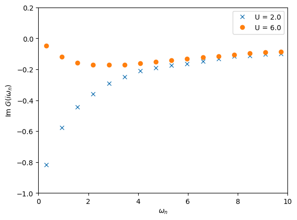
As you can see, the behavior of the imaginary part is very different for the two values of \(U\). When \(U\) is small, the system is a metal and the imaginary part extrapolated to zero goes to a finite value. Instead, for large \(U\), the system is a Mott insulator and the imaginary part goes to zero. The reason is that the extrapolation to zero is directly proportional to the density of states at the chemical potential. If the system is gapped, the density is zero; if the system is a metal, there is spectral weight and the density is finite. Therefore, even on the Matsubara axis, one has a way to decide if the system is metallic or not.
Exercise 3
Do the same exercise as above, but analyze the self-energy. The noise usually gets bigger for larger frequencies, so just focus on the first few Matsubara frequencies. There the noise should not be too important. Again, by looking at the extrapolation to zero frequency of the imaginary part of the self-energy, can you tell where the Mott transition happens?
Solution 3
We now do the same for the self-energy.
[4]:
A1 = HDFArchive("data/one_band/half-U2.00.h5", 'r')
A2 = HDFArchive("data/one_band/half-U6.00.h5", 'r')

# Plot the self-energy of the last iteration
oplot(A1['Sigma-9']['up'].imag, 'x', label='U = 2.0')
oplot(A2['Sigma-9']['up'].imag, 'o', label='U = 6.0')
plt.ylabel("$\\Sigma(i\\omega_n)$")

plt.xlim(0,5)
plt.ylim(-25,5)
plt.show()
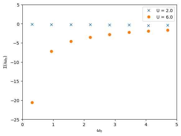
Exercise 4
A very useful quantity to measure the degree of correlation of a metal is the quasiparticle weight \(Z\). It is defined as
For a non-interacting metal \(Z=1\). As correlations appear, \(Z\) gradually gets smaller. It reaches 0 at the Mott transition. Make a plot of \(Z\) versus \(U\) for the Bethe lattice Hubbard model.
Hint: To access the values of \(\Sigma_\uparrow(i\omega_n)\), you can use S.Sigma['up'](n). This will be useful to numerically compute the derivative required to compute \(Z\).
Solution 4
We estimate the derivative using the following approximation
with \(\omega_0 = \pi / \beta\) being the first Matsubara frequency.
[5]:
import numpy as np
beta = 10
U_list = []
Z_list = []

for U in np.arange(1.0, 9.0):

    A = HDFArchive("data/one_band/half-U%.2f.h5"%U, 'r')
    Sigma = A['Sigma-9']

    Z = 1 / (1 - (Sigma['up'](0)[0,0].imag * beta / np.pi))
    U_list.append(U)
    Z_list.append(Z)

plt.plot(U_list, Z_list, '-o')
plt.xlabel('U')
plt.ylabel('Z')
plt.show()
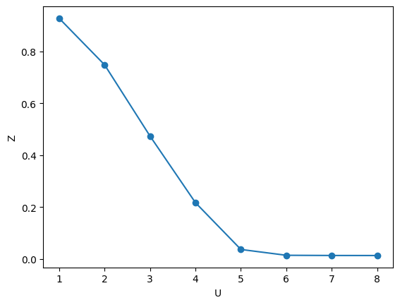
Exercise 5
Go back to your IPT code and try to modify it to extract the \(Z\) versus \(U\) curve. Compare this to the result you found in Exercise 4. Is the critical \(U\) for the Mott transition similar to the one you found using CTHYB?
Solution 5
This is just the same script as we had earlier. We just add a couple of lines to extract \(Z\).
[6]:
from triqs.gfs import *
from triqs.plot.mpl_interface import *

class IPTSolver:
    def __init__(self, beta):
        self.beta = beta

        # Matsubara frequency Green's functions
        iw_mesh = MeshImFreq(beta=beta, statistic='Fermion', n_iw=1001)
        self.G_iw = Gf(mesh=iw_mesh, target_shape=[1,1])
        self.G0_iw = self.G_iw.copy() # self.G0 will be set by the user after initialization
        self.Sigma_iw = self.G_iw.copy()

        # Imaginary time
        tau_mesh = MeshImTime(beta=beta, statistic='Fermion', n_tau=10001)
        self.G0_tau = Gf(mesh=tau_mesh, target_shape=[1,1])
        self.Sigma_tau = self.G0_tau.copy()

    def solve(self, U):
        self.G0_tau << Fourier(self.G0_iw)
        self.Sigma_tau << (U**2) * self.G0_tau * self.G0_tau * self.G0_tau
        self.Sigma_iw << Fourier(self.Sigma_tau)

        # Dyson
        self.G_iw << inverse(inverse(self.G0_iw) - self.Sigma_iw)

t = 1.0
beta = 10
n_loops = 30

S = IPTSolver(beta = beta)

U_list2 = []
Z_list2 = []

for U in np.arange(0.0, 9.0):

    S.G_iw << SemiCircular(2*t)
    for i in range(n_loops):

        S.G0_iw << inverse( iOmega_n - t**2 * S.G_iw )
        S.solve(U = U)


    Z = 1 / (1 - (S.Sigma_iw(0)[0,0].imag * beta / np.pi))
    U_list2.append(U)
    Z_list2.append(Z)

    print(Z)

plt.plot(U_list2, Z_list2, '-o', label='IPT')
plt.plot(U_list, Z_list, '-x', label='CTQMC')
plt.xlabel('U')
plt.ylabel('Z')
plt.legend()
plt.show()
1.0
0.9247647801661106
0.7405705430914762
0.5233633052723701
0.3175449850329105
0.048491181125403064
0.01758405717600884
0.010908997591308924
0.0076583553369136016
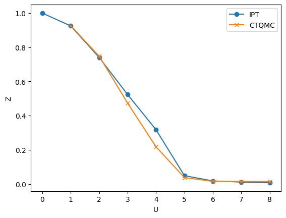
Exercise 6
Try to analytically continue the Green’s function on the real axis using the Pade approximation. What can you say about the result?
Solution 6
[7]:
from math import pi

with HDFArchive("data/one_band/half-U4.00.h5", 'r') as A:
    g = A['G-9']['up'][0,0]

w_mesh = MeshReFreq(window=(-5,5), n_w=1000)
g_real = Gf(mesh=w_mesh, target_shape=[])
g_real.set_from_pade(g)
oplot(-g_real.imag/pi, name=r"$\rho$")
plt.show()
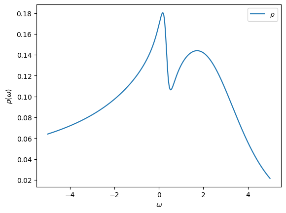
The result is completely wrong. This is because of the noise in the Monte Carlo data. One would have to make much longer runs in order to reduce the error bars. The Pade approximation can be used only on very accurate data. When the noise is still quite large, one has to use different analytical continuation methods, like MaxEnt, which produces the following spectral function:
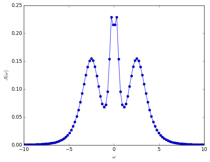
Regardless of which package you use for MaxEnt, it is very important to remember that there are some important knobs with which one can play in MaxEnt that can substantially change the results, and so one must be very careful in its use!
Exercise 7
In the last exercise we will analyze the impurity multiplets, the many-body states and their occupancies, using the CTHYB solver. To do this, we instruct the solver to measure the many-body density matrix of the impurity during sampling. This can be done at almost no additional numerical cost in CTHYB by passing the options measure_density_matrix = True and use_norm_as_weight = True to the solve call of the solver.
Write a small script that measures the impurity density matrix for two U-values (metallic and insulating) and analyzes/compares the two solutions by saving the solver object after convergence is reached for both values. Then you can access the density matrix as S.density_matrix. We provide a function to analyze the multiplets within CTHYB: triqs_cthyb.multiplet_tools.multiplet_analysis. Have a look at the
documentation to better understand how to use it. Use the code from exercise one to do this by extending it.
The function multiplet_analysis will also characterize each impurity many-body state with its quantum numbers. What is the characteristic feature in the multiplet structure of the Mott insulating state?
Tip: By default, printing a panda’s data frame shows all stored multiplets sorted by occupation probability.
[8]:
# Parameters of the model
t = 1.0
beta = 10
n_loops = 10

# Construct the impurity solver
S = Solver(beta = beta, gf_struct = [('up',1), ('down',1)] )

# run metallic U
U = 2.0

# This is a first guess for G
S.G_iw << SemiCircular(2*t)

# DMFT loop with self-consistency
for i in range(n_loops):
    print("\n\nIteration = %i / %i" % (i+1, n_loops))

    # Symmetrize the Green's function and use self-consistency
    g = 0.5 * ( S.G_iw['up'] + S.G_iw['down'] )
    for name, g0 in S.G0_iw:
        g0 << inverse( iOmega_n + U/2.0 - t**2 * g )

    # Solve the impurity problem
    S.solve(h_int = U * n('up',0) * n('down',0),   # Local Hamiltonian
        n_cycles  = 10000,                           # Number of QMC cycles
        n_warmup_cycles = 5000,                      # Warmup cycles
        measure_density_matrix = True,
        use_norm_as_weight = True
        )

solver_U_met = S

################################

U = 8.0
S = Solver(beta = beta, gf_struct = [('up',1), ('down',1)] )
# This is a first guess for G
S.G_iw << SemiCircular(2*t)

# DMFT loop with self-consistency
for i in range(n_loops):
    print("\n\nIteration = %i / %i" % (i+1, n_loops))

    # Symmetrize the Green's function and use self-consistency
    g = 0.5 * ( S.G_iw['up'] + S.G_iw['down'] )
    for name, g0 in S.G0_iw:
        g0 << inverse( iOmega_n + U/2.0 - t**2 * g )

    # Solve the impurity problem
    S.solve(h_int = U * n('up',0) * n('down',0),   # Local Hamiltonian
        n_cycles  = 10000,                         # Number of QMC cycles
        n_warmup_cycles = 5000,                    # Warmup cycles
        measure_density_matrix = True,
        use_norm_as_weight = True
        )

solver_U_ins = S
Iteration = 1 / 10

╔╦╗╦═╗╦╔═╗ ╔═╗  ┌─┐┌┬┐┬ ┬┬ ┬┌┐
 ║ ╠╦╝║║═╬╗╚═╗  │   │ ├─┤└┬┘├┴┐
 ╩ ╩╚═╩╚═╝╚╚═╝  └─┘ ┴ ┴ ┴ ┴ └─┘

The local Hamiltonian of the problem:
-1*c_dag('down',0)*c('down',0) + -1*c_dag('up',0)*c('up',0) + 2*c_dag('down',0)*c_dag('up',0)*c('up',0)*c('down',0)
Using autopartition algorithm to partition the local Hilbert space
Found 4 subspaces.
[Rank 0] Performing warmup phase...
[Rank 0] 08:07:56  28.06% done, ETA 00:00:00, cycle 1403 of 5000, 1.40e+04 cycles/sec
[Rank 0] 08:07:57 100.00% done, ETA 00:00:00, cycle 5000 of 5000, 1.36e+04 cycles/sec
[Rank 0] Performing accumulation phase...
[Rank 0] 08:07:57  13.58% done, ETA 00:00:00, cycle 1358 of 10000, 1.36e+04 cycles/sec
[Rank 0] 08:07:57 100.00% done, ETA 00:00:00, cycle 10000 of 10000, 1.33e+04 cycles/sec
[Rank 0] Collect results: Waiting for all MPI processes to finish accumulating...

[Rank 0] Warmup duration: 0.3676 seconds [00:00:00]
[Rank 0] Simulation duration: 0.7543 seconds [00:00:00]
[Rank 0] Number of measures: 10000
[Rank 0] Cycles (measures) / second: 1.33e+04
[Rank 0] Measurement durations (total = 0.0160):
[Rank 0]   Measure Auto-correlation time: Duration = 0.0010
[Rank 0]   Measure Average order: Duration = 0.0002
[Rank 0]   Measure Average sign: Duration = 0.0002
[Rank 0]   Measure Density Matrix for local static observable: Duration = 0.0118
[Rank 0]   Measure G_tau measure: Duration = 0.0027
[Rank 0] Move durations (total = 0.7114):
[Rank 0]   Move set Insert two operators: Duration = 0.1114
[Rank 0]     Move Insert Delta_up: Duration = 0.0517
[Rank 0]     Move Insert Delta_down: Duration = 0.0519
[Rank 0]   Move set Remove two operators: Duration = 0.1031
[Rank 0]     Move Remove Delta_up: Duration = 0.0477
[Rank 0]     Move Remove Delta_down: Duration = 0.0477
[Rank 0]   Move set Insert four operators: Duration = 0.1402
[Rank 0]     Move Insert Delta_up_up: Duration = 0.0374
[Rank 0]     Move Insert Delta_up_down: Duration = 0.0284
[Rank 0]     Move Insert Delta_down_up: Duration = 0.0287
[Rank 0]     Move Insert Delta_down_down: Duration = 0.0372
[Rank 0]   Move set Remove four operators: Duration = 0.0914
[Rank 0]     Move Remove Delta_up_up: Duration = 0.0172
[Rank 0]     Move Remove Delta_up_down: Duration = 0.0244
[Rank 0]     Move Remove Delta_down_up: Duration = 0.0241
[Rank 0]     Move Remove Delta_down_down: Duration = 0.0172
[Rank 0]   Move Shift one operator: Duration = 0.2654
[Rank 0] Move statistics:
[Rank 0]   Move set Insert two operators: Proposed = 99920, Accepted = 12643, Rate = 0.1265
[Rank 0]     Move Insert Delta_up: Proposed = 49884, Accepted = 6331, Rate = 0.1269
[Rank 0]     Move Insert Delta_down: Proposed = 50036, Accepted = 6312, Rate = 0.1261
[Rank 0]   Move set Remove two operators: Proposed = 99826, Accepted = 12597, Rate = 0.1262
[Rank 0]     Move Remove Delta_up: Proposed = 50052, Accepted = 6308, Rate = 0.1260
[Rank 0]     Move Remove Delta_down: Proposed = 49774, Accepted = 6289, Rate = 0.1264
[Rank 0]   Move set Insert four operators: Proposed = 99905, Accepted = 2468, Rate = 0.0247
[Rank 0]     Move Insert Delta_up_up: Proposed = 25091, Accepted = 690, Rate = 0.0275
[Rank 0]     Move Insert Delta_up_down: Proposed = 24858, Accepted = 536, Rate = 0.0216
[Rank 0]     Move Insert Delta_down_up: Proposed = 25006, Accepted = 570, Rate = 0.0228
[Rank 0]     Move Insert Delta_down_down: Proposed = 24950, Accepted = 672, Rate = 0.0269
[Rank 0]   Move set Remove four operators: Proposed = 99861, Accepted = 2491, Rate = 0.0249
[Rank 0]     Move Remove Delta_up_up: Proposed = 24749, Accepted = 702, Rate = 0.0284
[Rank 0]     Move Remove Delta_up_down: Proposed = 25187, Accepted = 575, Rate = 0.0228
[Rank 0]     Move Remove Delta_down_up: Proposed = 24955, Accepted = 532, Rate = 0.0213
[Rank 0]     Move Remove Delta_down_down: Proposed = 24970, Accepted = 682, Rate = 0.0273
[Rank 0]   Move Shift one operator: Proposed = 100488, Accepted = 69717, Rate = 0.6938

Total number of measures: 10000
Total cycles (measures) / second: 1.33e+04
Average sign: 1
Average order: 7.5979
Auto-correlation time: 2.56532 cycles


Iteration = 2 / 10

╔╦╗╦═╗╦╔═╗ ╔═╗  ┌─┐┌┬┐┬ ┬┬ ┬┌┐
 ║ ╠╦╝║║═╬╗╚═╗  │   │ ├─┤└┬┘├┴┐
 ╩ ╩╚═╩╚═╝╚╚═╝  └─┘ ┴ ┴ ┴ ┴ └─┘

The local Hamiltonian of the problem:
-1*c_dag('down',0)*c('down',0) + -1*c_dag('up',0)*c('up',0) + 2*c_dag('down',0)*c_dag('up',0)*c('up',0)*c('down',0)
Using autopartition algorithm to partition the local Hilbert space
Found 4 subspaces.
[Rank 0] Performing warmup phase...
[Rank 0] 08:07:57  25.92% done, ETA 00:00:00, cycle 1296 of 5000, 1.30e+04 cycles/sec
[Rank 0] 08:07:58 100.00% done, ETA 00:00:00, cycle 5000 of 5000, 1.34e+04 cycles/sec
[Rank 0] Performing accumulation phase...
[Rank 0] 08:07:58  12.16% done, ETA 00:00:00, cycle 1216 of 10000, 1.22e+04 cycles/sec
[Rank 0] 08:07:58 100.00% done, ETA 00:00:00, cycle 10000 of 10000, 1.31e+04 cycles/sec
[Rank 0] Collect results: Waiting for all MPI processes to finish accumulating...

[Rank 0] Warmup duration: 0.3720 seconds [00:00:00]
[Rank 0] Simulation duration: 0.7649 seconds [00:00:00]
[Rank 0] Number of measures: 10000
[Rank 0] Cycles (measures) / second: 1.31e+04
[Rank 0] Measurement durations (total = 0.0161):
[Rank 0]   Measure Auto-correlation time: Duration = 0.0010
[Rank 0]   Measure Average order: Duration = 0.0003
[Rank 0]   Measure Average sign: Duration = 0.0002
[Rank 0]   Measure Density Matrix for local static observable: Duration = 0.0120
[Rank 0]   Measure G_tau measure: Duration = 0.0026
[Rank 0] Move durations (total = 0.7211):
[Rank 0]   Move set Insert two operators: Duration = 0.1148
[Rank 0]     Move Insert Delta_up: Duration = 0.0531
[Rank 0]     Move Insert Delta_down: Duration = 0.0536
[Rank 0]   Move set Remove two operators: Duration = 0.1057
[Rank 0]     Move Remove Delta_up: Duration = 0.0489
[Rank 0]     Move Remove Delta_down: Duration = 0.0487
[Rank 0]   Move set Insert four operators: Duration = 0.1440
[Rank 0]     Move Insert Delta_up_up: Duration = 0.0385
[Rank 0]     Move Insert Delta_up_down: Duration = 0.0293
[Rank 0]     Move Insert Delta_down_up: Duration = 0.0294
[Rank 0]     Move Insert Delta_down_down: Duration = 0.0383
[Rank 0]   Move set Remove four operators: Duration = 0.0922
[Rank 0]     Move Remove Delta_up_up: Duration = 0.0172
[Rank 0]     Move Remove Delta_up_down: Duration = 0.0248
[Rank 0]     Move Remove Delta_down_up: Duration = 0.0246
[Rank 0]     Move Remove Delta_down_down: Duration = 0.0172
[Rank 0]   Move Shift one operator: Duration = 0.2643
[Rank 0] Move statistics:
[Rank 0]   Move set Insert two operators: Proposed = 100049, Accepted = 13044, Rate = 0.1304
[Rank 0]     Move Insert Delta_up: Proposed = 49820, Accepted = 6496, Rate = 0.1304
[Rank 0]     Move Insert Delta_down: Proposed = 50229, Accepted = 6548, Rate = 0.1304
[Rank 0]   Move set Remove two operators: Proposed = 99766, Accepted = 12920, Rate = 0.1295
[Rank 0]     Move Remove Delta_up: Proposed = 49904, Accepted = 6492, Rate = 0.1301
[Rank 0]     Move Remove Delta_down: Proposed = 49862, Accepted = 6428, Rate = 0.1289
[Rank 0]   Move set Insert four operators: Proposed = 99991, Accepted = 2675, Rate = 0.0268
[Rank 0]     Move Insert Delta_up_up: Proposed = 25086, Accepted = 764, Rate = 0.0305
[Rank 0]     Move Insert Delta_up_down: Proposed = 24940, Accepted = 610, Rate = 0.0245
[Rank 0]     Move Insert Delta_down_up: Proposed = 24940, Accepted = 615, Rate = 0.0247
[Rank 0]     Move Insert Delta_down_down: Proposed = 25025, Accepted = 686, Rate = 0.0274
[Rank 0]   Move set Remove four operators: Proposed = 99834, Accepted = 2737, Rate = 0.0274
[Rank 0]     Move Remove Delta_up_up: Proposed = 24802, Accepted = 745, Rate = 0.0300
[Rank 0]     Move Remove Delta_up_down: Proposed = 25111, Accepted = 657, Rate = 0.0262
[Rank 0]     Move Remove Delta_down_up: Proposed = 24982, Accepted = 613, Rate = 0.0245
[Rank 0]     Move Remove Delta_down_down: Proposed = 24939, Accepted = 722, Rate = 0.0290
[Rank 0]   Move Shift one operator: Proposed = 100360, Accepted = 67430, Rate = 0.6719

Total number of measures: 10000
Total cycles (measures) / second: 1.31e+04
Average sign: 1
Average order: 7.2697
Auto-correlation time: 2.44844 cycles


Iteration = 3 / 10

╔╦╗╦═╗╦╔═╗ ╔═╗  ┌─┐┌┬┐┬ ┬┬ ┬┌┐
 ║ ╠╦╝║║═╬╗╚═╗  │   │ ├─┤└┬┘├┴┐
 ╩ ╩╚═╩╚═╝╚╚═╝  └─┘ ┴ ┴ ┴ ┴ └─┘

The local Hamiltonian of the problem:
-1*c_dag('down',0)*c('down',0) + -1*c_dag('up',0)*c('up',0) + 2*c_dag('down',0)*c_dag('up',0)*c('up',0)*c('down',0)
Using autopartition algorithm to partition the local Hilbert space
Found 4 subspaces.
[Rank 0] Performing warmup phase...
[Rank 0] 08:07:59  27.24% done, ETA 00:00:00, cycle 1362 of 5000, 1.36e+04 cycles/sec
[Rank 0] 08:07:59 100.00% done, ETA 00:00:00, cycle 5000 of 5000, 1.38e+04 cycles/sec
[Rank 0] Performing accumulation phase...
[Rank 0] 08:07:59  12.94% done, ETA 00:00:00, cycle 1294 of 10000, 1.29e+04 cycles/sec
[Rank 0] 08:08:00 100.00% done, ETA 00:00:00, cycle 10000 of 10000, 1.33e+04 cycles/sec
[Rank 0] Collect results: Waiting for all MPI processes to finish accumulating...

[Rank 0] Warmup duration: 0.3612 seconds [00:00:00]
[Rank 0] Simulation duration: 0.7530 seconds [00:00:00]
[Rank 0] Number of measures: 10000
[Rank 0] Cycles (measures) / second: 1.33e+04
[Rank 0] Measurement durations (total = 0.0158):
[Rank 0]   Measure Auto-correlation time: Duration = 0.0010
[Rank 0]   Measure Average order: Duration = 0.0002
[Rank 0]   Measure Average sign: Duration = 0.0002
[Rank 0]   Measure Density Matrix for local static observable: Duration = 0.0118
[Rank 0]   Measure G_tau measure: Duration = 0.0026
[Rank 0] Move durations (total = 0.7104):
[Rank 0]   Move set Insert two operators: Duration = 0.1125
[Rank 0]     Move Insert Delta_up: Duration = 0.0518
[Rank 0]     Move Insert Delta_down: Duration = 0.0526
[Rank 0]   Move set Remove two operators: Duration = 0.1031
[Rank 0]     Move Remove Delta_up: Duration = 0.0474
[Rank 0]     Move Remove Delta_down: Duration = 0.0478
[Rank 0]   Move set Insert four operators: Duration = 0.1404
[Rank 0]     Move Insert Delta_up_up: Duration = 0.0374
[Rank 0]     Move Insert Delta_up_down: Duration = 0.0285
[Rank 0]     Move Insert Delta_down_up: Duration = 0.0287
[Rank 0]     Move Insert Delta_down_down: Duration = 0.0374
[Rank 0]   Move set Remove four operators: Duration = 0.0911
[Rank 0]     Move Remove Delta_up_up: Duration = 0.0170
[Rank 0]     Move Remove Delta_up_down: Duration = 0.0244
[Rank 0]     Move Remove Delta_down_up: Duration = 0.0240
[Rank 0]     Move Remove Delta_down_down: Duration = 0.0174
[Rank 0]   Move Shift one operator: Duration = 0.2632
[Rank 0] Move statistics:
[Rank 0]   Move set Insert two operators: Proposed = 100156, Accepted = 12949, Rate = 0.1293
[Rank 0]     Move Insert Delta_up: Proposed = 50104, Accepted = 6394, Rate = 0.1276
[Rank 0]     Move Insert Delta_down: Proposed = 50052, Accepted = 6555, Rate = 0.1310
[Rank 0]   Move set Remove two operators: Proposed = 99565, Accepted = 12748, Rate = 0.1280
[Rank 0]     Move Remove Delta_up: Proposed = 49903, Accepted = 6307, Rate = 0.1264
[Rank 0]     Move Remove Delta_down: Proposed = 49662, Accepted = 6441, Rate = 0.1297
[Rank 0]   Move set Insert four operators: Proposed = 100062, Accepted = 2514, Rate = 0.0251
[Rank 0]     Move Insert Delta_up_up: Proposed = 25071, Accepted = 686, Rate = 0.0274
[Rank 0]     Move Insert Delta_up_down: Proposed = 24931, Accepted = 547, Rate = 0.0219
[Rank 0]     Move Insert Delta_down_up: Proposed = 24995, Accepted = 586, Rate = 0.0234
[Rank 0]     Move Insert Delta_down_down: Proposed = 25065, Accepted = 695, Rate = 0.0277
[Rank 0]   Move set Remove four operators: Proposed = 99869, Accepted = 2613, Rate = 0.0262
[Rank 0]     Move Remove Delta_up_up: Proposed = 24888, Accepted = 694, Rate = 0.0279
[Rank 0]     Move Remove Delta_up_down: Proposed = 25082, Accepted = 613, Rate = 0.0244
[Rank 0]     Move Remove Delta_down_up: Proposed = 24870, Accepted = 591, Rate = 0.0238
[Rank 0]     Move Remove Delta_down_down: Proposed = 25029, Accepted = 715, Rate = 0.0286
[Rank 0]   Move Shift one operator: Proposed = 100348, Accepted = 69016, Rate = 0.6878

Total number of measures: 10000
Total cycles (measures) / second: 1.33e+04
Average sign: 1
Average order: 7.5226
Auto-correlation time: 2.21394 cycles


Iteration = 4 / 10

╔╦╗╦═╗╦╔═╗ ╔═╗  ┌─┐┌┬┐┬ ┬┬ ┬┌┐
 ║ ╠╦╝║║═╬╗╚═╗  │   │ ├─┤└┬┘├┴┐
 ╩ ╩╚═╩╚═╝╚╚═╝  └─┘ ┴ ┴ ┴ ┴ └─┘

The local Hamiltonian of the problem:
-1*c_dag('down',0)*c('down',0) + -1*c_dag('up',0)*c('up',0) + 2*c_dag('down',0)*c_dag('up',0)*c('up',0)*c('down',0)
Using autopartition algorithm to partition the local Hilbert space
Found 4 subspaces.
[Rank 0] Performing warmup phase...
[Rank 0] 08:08:00  27.64% done, ETA 00:00:00, cycle 1382 of 5000, 1.38e+04 cycles/sec
[Rank 0] 08:08:00 100.00% done, ETA 00:00:00, cycle 5000 of 5000, 1.36e+04 cycles/sec
[Rank 0] Performing accumulation phase...
[Rank 0] 08:08:00  13.90% done, ETA 00:00:00, cycle 1390 of 10000, 1.39e+04 cycles/sec
[Rank 0] 08:08:01 100.00% done, ETA 00:00:00, cycle 10000 of 10000, 1.37e+04 cycles/sec
[Rank 0] Collect results: Waiting for all MPI processes to finish accumulating...

[Rank 0] Warmup duration: 0.3681 seconds [00:00:00]
[Rank 0] Simulation duration: 0.7325 seconds [00:00:00]
[Rank 0] Number of measures: 10000
[Rank 0] Cycles (measures) / second: 1.37e+04
[Rank 0] Measurement durations (total = 0.0154):
[Rank 0]   Measure Auto-correlation time: Duration = 0.0010
[Rank 0]   Measure Average order: Duration = 0.0002
[Rank 0]   Measure Average sign: Duration = 0.0002
[Rank 0]   Measure Density Matrix for local static observable: Duration = 0.0115
[Rank 0]   Measure G_tau measure: Duration = 0.0025
[Rank 0] Move durations (total = 0.6906):
[Rank 0]   Move set Insert two operators: Duration = 0.1094
[Rank 0]     Move Insert Delta_up: Duration = 0.0506
[Rank 0]     Move Insert Delta_down: Duration = 0.0512
[Rank 0]   Move set Remove two operators: Duration = 0.1006
[Rank 0]     Move Remove Delta_up: Duration = 0.0466
[Rank 0]     Move Remove Delta_down: Duration = 0.0464
[Rank 0]   Move set Insert four operators: Duration = 0.1375
[Rank 0]     Move Insert Delta_up_up: Duration = 0.0367
[Rank 0]     Move Insert Delta_up_down: Duration = 0.0279
[Rank 0]     Move Insert Delta_down_up: Duration = 0.0282
[Rank 0]     Move Insert Delta_down_down: Duration = 0.0365
[Rank 0]   Move set Remove four operators: Duration = 0.0883
[Rank 0]     Move Remove Delta_up_up: Duration = 0.0163
[Rank 0]     Move Remove Delta_up_down: Duration = 0.0237
[Rank 0]     Move Remove Delta_down_up: Duration = 0.0235
[Rank 0]     Move Remove Delta_down_down: Duration = 0.0168
[Rank 0]   Move Shift one operator: Duration = 0.2548
[Rank 0] Move statistics:
[Rank 0]   Move set Insert two operators: Proposed = 100104, Accepted = 12911, Rate = 0.1290
[Rank 0]     Move Insert Delta_up: Proposed = 49921, Accepted = 6419, Rate = 0.1286
[Rank 0]     Move Insert Delta_down: Proposed = 50183, Accepted = 6492, Rate = 0.1294
[Rank 0]   Move set Remove two operators: Proposed = 99495, Accepted = 12869, Rate = 0.1293
[Rank 0]     Move Remove Delta_up: Proposed = 49834, Accepted = 6452, Rate = 0.1295
[Rank 0]     Move Remove Delta_down: Proposed = 49661, Accepted = 6417, Rate = 0.1292
[Rank 0]   Move set Insert four operators: Proposed = 100126, Accepted = 2666, Rate = 0.0266
[Rank 0]     Move Insert Delta_up_up: Proposed = 25153, Accepted = 742, Rate = 0.0295
[Rank 0]     Move Insert Delta_up_down: Proposed = 24902, Accepted = 582, Rate = 0.0234
[Rank 0]     Move Insert Delta_down_up: Proposed = 25053, Accepted = 637, Rate = 0.0254
[Rank 0]     Move Insert Delta_down_down: Proposed = 25018, Accepted = 705, Rate = 0.0282
[Rank 0]   Move set Remove four operators: Proposed = 99820, Accepted = 2688, Rate = 0.0269
[Rank 0]     Move Remove Delta_up_up: Proposed = 24756, Accepted = 725, Rate = 0.0293
[Rank 0]     Move Remove Delta_up_down: Proposed = 25155, Accepted = 614, Rate = 0.0244
[Rank 0]     Move Remove Delta_down_up: Proposed = 24875, Accepted = 607, Rate = 0.0244
[Rank 0]     Move Remove Delta_down_down: Proposed = 25034, Accepted = 742, Rate = 0.0296
[Rank 0]   Move Shift one operator: Proposed = 100455, Accepted = 68115, Rate = 0.6781

Total number of measures: 10000
Total cycles (measures) / second: 1.37e+04
Average sign: 1
Average order: 7.3514
Auto-correlation time: 2.67965 cycles


Iteration = 5 / 10

╔╦╗╦═╗╦╔═╗ ╔═╗  ┌─┐┌┬┐┬ ┬┬ ┬┌┐
 ║ ╠╦╝║║═╬╗╚═╗  │   │ ├─┤└┬┘├┴┐
 ╩ ╩╚═╩╚═╝╚╚═╝  └─┘ ┴ ┴ ┴ ┴ └─┘

The local Hamiltonian of the problem:
-1*c_dag('down',0)*c('down',0) + -1*c_dag('up',0)*c('up',0) + 2*c_dag('down',0)*c_dag('up',0)*c('up',0)*c('down',0)
Using autopartition algorithm to partition the local Hilbert space
Found 4 subspaces.
[Rank 0] Performing warmup phase...
[Rank 0] 08:08:01  27.52% done, ETA 00:00:00, cycle 1376 of 5000, 1.38e+04 cycles/sec
[Rank 0] 08:08:01 100.00% done, ETA 00:00:00, cycle 5000 of 5000, 1.33e+04 cycles/sec
[Rank 0] Performing accumulation phase...
[Rank 0] 08:08:01  14.30% done, ETA 00:00:00, cycle 1430 of 10000, 1.43e+04 cycles/sec
[Rank 0] 08:08:02 100.00% done, ETA 00:00:00, cycle 10000 of 10000, 1.39e+04 cycles/sec
[Rank 0] Collect results: Waiting for all MPI processes to finish accumulating...

[Rank 0] Warmup duration: 0.3746 seconds [00:00:00]
[Rank 0] Simulation duration: 0.7208 seconds [00:00:00]
[Rank 0] Number of measures: 10000
[Rank 0] Cycles (measures) / second: 1.39e+04
[Rank 0] Measurement durations (total = 0.0150):
[Rank 0]   Measure Auto-correlation time: Duration = 0.0010
[Rank 0]   Measure Average order: Duration = 0.0002
[Rank 0]   Measure Average sign: Duration = 0.0002
[Rank 0]   Measure Density Matrix for local static observable: Duration = 0.0112
[Rank 0]   Measure G_tau measure: Duration = 0.0024
[Rank 0] Move durations (total = 0.6800):
[Rank 0]   Move set Insert two operators: Duration = 0.1081
[Rank 0]     Move Insert Delta_up: Duration = 0.0498
[Rank 0]     Move Insert Delta_down: Duration = 0.0507
[Rank 0]   Move set Remove two operators: Duration = 0.0996
[Rank 0]     Move Remove Delta_up: Duration = 0.0458
[Rank 0]     Move Remove Delta_down: Duration = 0.0462
[Rank 0]   Move set Insert four operators: Duration = 0.1354
[Rank 0]     Move Insert Delta_up_up: Duration = 0.0361
[Rank 0]     Move Insert Delta_up_down: Duration = 0.0277
[Rank 0]     Move Insert Delta_down_up: Duration = 0.0280
[Rank 0]     Move Insert Delta_down_down: Duration = 0.0358
[Rank 0]   Move set Remove four operators: Duration = 0.0869
[Rank 0]     Move Remove Delta_up_up: Duration = 0.0163
[Rank 0]     Move Remove Delta_up_down: Duration = 0.0231
[Rank 0]     Move Remove Delta_down_up: Duration = 0.0231
[Rank 0]     Move Remove Delta_down_down: Duration = 0.0164
[Rank 0]   Move Shift one operator: Duration = 0.2500
[Rank 0] Move statistics:
[Rank 0]   Move set Insert two operators: Proposed = 99893, Accepted = 13111, Rate = 0.1313
[Rank 0]     Move Insert Delta_up: Proposed = 49788, Accepted = 6487, Rate = 0.1303
[Rank 0]     Move Insert Delta_down: Proposed = 50105, Accepted = 6624, Rate = 0.1322
[Rank 0]   Move set Remove two operators: Proposed = 99851, Accepted = 13106, Rate = 0.1313
[Rank 0]     Move Remove Delta_up: Proposed = 50024, Accepted = 6498, Rate = 0.1299
[Rank 0]     Move Remove Delta_down: Proposed = 49827, Accepted = 6608, Rate = 0.1326
[Rank 0]   Move set Insert four operators: Proposed = 99826, Accepted = 2731, Rate = 0.0274
[Rank 0]     Move Insert Delta_up_up: Proposed = 25125, Accepted = 716, Rate = 0.0285
[Rank 0]     Move Insert Delta_up_down: Proposed = 24838, Accepted = 663, Rate = 0.0267
[Rank 0]     Move Insert Delta_down_up: Proposed = 24978, Accepted = 676, Rate = 0.0271
[Rank 0]     Move Insert Delta_down_down: Proposed = 24885, Accepted = 676, Rate = 0.0272
[Rank 0]   Move set Remove four operators: Proposed = 99907, Accepted = 2732, Rate = 0.0273
[Rank 0]     Move Remove Delta_up_up: Proposed = 24835, Accepted = 765, Rate = 0.0308
[Rank 0]     Move Remove Delta_up_down: Proposed = 25098, Accepted = 614, Rate = 0.0245
[Rank 0]     Move Remove Delta_down_up: Proposed = 24909, Accepted = 613, Rate = 0.0246
[Rank 0]     Move Remove Delta_down_down: Proposed = 25065, Accepted = 740, Rate = 0.0295
[Rank 0]   Move Shift one operator: Proposed = 100523, Accepted = 68365, Rate = 0.6801

Total number of measures: 10000
Total cycles (measures) / second: 1.39e+04
Average sign: 1
Average order: 7.348
Auto-correlation time: 2.65435 cycles


Iteration = 6 / 10

╔╦╗╦═╗╦╔═╗ ╔═╗  ┌─┐┌┬┐┬ ┬┬ ┬┌┐
 ║ ╠╦╝║║═╬╗╚═╗  │   │ ├─┤└┬┘├┴┐
 ╩ ╩╚═╩╚═╝╚╚═╝  └─┘ ┴ ┴ ┴ ┴ └─┘

The local Hamiltonian of the problem:
-1*c_dag('down',0)*c('down',0) + -1*c_dag('up',0)*c('up',0) + 2*c_dag('down',0)*c_dag('up',0)*c('up',0)*c('down',0)
Using autopartition algorithm to partition the local Hilbert space
Found 4 subspaces.
[Rank 0] Performing warmup phase...
[Rank 0] 08:08:02  24.64% done, ETA 00:00:00, cycle 1232 of 5000, 1.23e+04 cycles/sec
[Rank 0] 08:08:02 100.00% done, ETA 00:00:00, cycle 5000 of 5000, 1.36e+04 cycles/sec
[Rank 0] Performing accumulation phase...
[Rank 0] 08:08:02  14.04% done, ETA 00:00:00, cycle 1404 of 10000, 1.40e+04 cycles/sec
[Rank 0] 08:08:03 100.00% done, ETA 00:00:00, cycle 10000 of 10000, 1.34e+04 cycles/sec
[Rank 0] Collect results: Waiting for all MPI processes to finish accumulating...

[Rank 0] Warmup duration: 0.3672 seconds [00:00:00]
[Rank 0] Simulation duration: 0.7468 seconds [00:00:00]
[Rank 0] Number of measures: 10000
[Rank 0] Cycles (measures) / second: 1.34e+04
[Rank 0] Measurement durations (total = 0.0157):
[Rank 0]   Measure Auto-correlation time: Duration = 0.0010
[Rank 0]   Measure Average order: Duration = 0.0002
[Rank 0]   Measure Average sign: Duration = 0.0002
[Rank 0]   Measure Density Matrix for local static observable: Duration = 0.0117
[Rank 0]   Measure G_tau measure: Duration = 0.0026
[Rank 0] Move durations (total = 0.7045):
[Rank 0]   Move set Insert two operators: Duration = 0.1115
[Rank 0]     Move Insert Delta_up: Duration = 0.0520
[Rank 0]     Move Insert Delta_down: Duration = 0.0517
[Rank 0]   Move set Remove two operators: Duration = 0.1031
[Rank 0]     Move Remove Delta_up: Duration = 0.0477
[Rank 0]     Move Remove Delta_down: Duration = 0.0475
[Rank 0]   Move set Insert four operators: Duration = 0.1399
[Rank 0]     Move Insert Delta_up_up: Duration = 0.0373
[Rank 0]     Move Insert Delta_up_down: Duration = 0.0286
[Rank 0]     Move Insert Delta_down_up: Duration = 0.0283
[Rank 0]     Move Insert Delta_down_down: Duration = 0.0374
[Rank 0]   Move set Remove four operators: Duration = 0.0904
[Rank 0]     Move Remove Delta_up_up: Duration = 0.0169
[Rank 0]     Move Remove Delta_up_down: Duration = 0.0241
[Rank 0]     Move Remove Delta_down_up: Duration = 0.0241
[Rank 0]     Move Remove Delta_down_down: Duration = 0.0170
[Rank 0]   Move Shift one operator: Duration = 0.2596
[Rank 0] Move statistics:
[Rank 0]   Move set Insert two operators: Proposed = 99931, Accepted = 12958, Rate = 0.1297
[Rank 0]     Move Insert Delta_up: Proposed = 49988, Accepted = 6569, Rate = 0.1314
[Rank 0]     Move Insert Delta_down: Proposed = 49943, Accepted = 6389, Rate = 0.1279
[Rank 0]   Move set Remove two operators: Proposed = 99774, Accepted = 12913, Rate = 0.1294
[Rank 0]     Move Remove Delta_up: Proposed = 49901, Accepted = 6511, Rate = 0.1305
[Rank 0]     Move Remove Delta_down: Proposed = 49873, Accepted = 6402, Rate = 0.1284
[Rank 0]   Move set Insert four operators: Proposed = 99917, Accepted = 2647, Rate = 0.0265
[Rank 0]     Move Insert Delta_up_up: Proposed = 25010, Accepted = 731, Rate = 0.0292
[Rank 0]     Move Insert Delta_up_down: Proposed = 24911, Accepted = 617, Rate = 0.0248
[Rank 0]     Move Insert Delta_down_up: Proposed = 25005, Accepted = 559, Rate = 0.0224
[Rank 0]     Move Insert Delta_down_down: Proposed = 24991, Accepted = 740, Rate = 0.0296
[Rank 0]   Move set Remove four operators: Proposed = 99751, Accepted = 2669, Rate = 0.0268
[Rank 0]     Move Remove Delta_up_up: Proposed = 24737, Accepted = 730, Rate = 0.0295
[Rank 0]     Move Remove Delta_up_down: Proposed = 25152, Accepted = 604, Rate = 0.0240
[Rank 0]     Move Remove Delta_down_up: Proposed = 24863, Accepted = 631, Rate = 0.0254
[Rank 0]     Move Remove Delta_down_down: Proposed = 24999, Accepted = 704, Rate = 0.0282
[Rank 0]   Move Shift one operator: Proposed = 100627, Accepted = 68288, Rate = 0.6786

Total number of measures: 10000
Total cycles (measures) / second: 1.34e+04
Average sign: 1
Average order: 7.4147
Auto-correlation time: 2.09005 cycles


Iteration = 7 / 10

╔╦╗╦═╗╦╔═╗ ╔═╗  ┌─┐┌┬┐┬ ┬┬ ┬┌┐
 ║ ╠╦╝║║═╬╗╚═╗  │   │ ├─┤└┬┘├┴┐
 ╩ ╩╚═╩╚═╝╚╚═╝  └─┘ ┴ ┴ ┴ ┴ └─┘

The local Hamiltonian of the problem:
-1*c_dag('down',0)*c('down',0) + -1*c_dag('up',0)*c('up',0) + 2*c_dag('down',0)*c_dag('up',0)*c('up',0)*c('down',0)
Using autopartition algorithm to partition the local Hilbert space
Found 4 subspaces.
[Rank 0] Performing warmup phase...
[Rank 0] 08:08:03  29.18% done, ETA 00:00:00, cycle 1459 of 5000, 1.46e+04 cycles/sec
[Rank 0] 08:08:03 100.00% done, ETA 00:00:00, cycle 5000 of 5000, 1.42e+04 cycles/sec
[Rank 0] Performing accumulation phase...
[Rank 0] 08:08:03  13.26% done, ETA 00:00:00, cycle 1326 of 10000, 1.33e+04 cycles/sec
[Rank 0] 08:08:04 100.00% done, ETA 00:00:00, cycle 10000 of 10000, 1.35e+04 cycles/sec
[Rank 0] Collect results: Waiting for all MPI processes to finish accumulating...

[Rank 0] Warmup duration: 0.3519 seconds [00:00:00]
[Rank 0] Simulation duration: 0.7404 seconds [00:00:00]
[Rank 0] Number of measures: 10000
[Rank 0] Cycles (measures) / second: 1.35e+04
[Rank 0] Measurement durations (total = 0.0156):
[Rank 0]   Measure Auto-correlation time: Duration = 0.0010
[Rank 0]   Measure Average order: Duration = 0.0002
[Rank 0]   Measure Average sign: Duration = 0.0002
[Rank 0]   Measure Density Matrix for local static observable: Duration = 0.0117
[Rank 0]   Measure G_tau measure: Duration = 0.0025
[Rank 0] Move durations (total = 0.6984):
[Rank 0]   Move set Insert two operators: Duration = 0.1107
[Rank 0]     Move Insert Delta_up: Duration = 0.0516
[Rank 0]     Move Insert Delta_down: Duration = 0.0514
[Rank 0]   Move set Remove two operators: Duration = 0.1025
[Rank 0]     Move Remove Delta_up: Duration = 0.0476
[Rank 0]     Move Remove Delta_down: Duration = 0.0472
[Rank 0]   Move set Insert four operators: Duration = 0.1388
[Rank 0]     Move Insert Delta_up_up: Duration = 0.0367
[Rank 0]     Move Insert Delta_up_down: Duration = 0.0284
[Rank 0]     Move Insert Delta_down_up: Duration = 0.0283
[Rank 0]     Move Insert Delta_down_down: Duration = 0.0370
[Rank 0]   Move set Remove four operators: Duration = 0.0896
[Rank 0]     Move Remove Delta_up_up: Duration = 0.0166
[Rank 0]     Move Remove Delta_up_down: Duration = 0.0241
[Rank 0]     Move Remove Delta_down_up: Duration = 0.0238
[Rank 0]     Move Remove Delta_down_down: Duration = 0.0168
[Rank 0]   Move Shift one operator: Duration = 0.2569
[Rank 0] Move statistics:
[Rank 0]   Move set Insert two operators: Proposed = 100017, Accepted = 13114, Rate = 0.1311
[Rank 0]     Move Insert Delta_up: Proposed = 49847, Accepted = 6639, Rate = 0.1332
[Rank 0]     Move Insert Delta_down: Proposed = 50170, Accepted = 6475, Rate = 0.1291
[Rank 0]   Move set Remove two operators: Proposed = 99902, Accepted = 13080, Rate = 0.1309
[Rank 0]     Move Remove Delta_up: Proposed = 49917, Accepted = 6563, Rate = 0.1315
[Rank 0]     Move Remove Delta_down: Proposed = 49985, Accepted = 6517, Rate = 0.1304
[Rank 0]   Move set Insert four operators: Proposed = 99893, Accepted = 2725, Rate = 0.0273
[Rank 0]     Move Insert Delta_up_up: Proposed = 24974, Accepted = 728, Rate = 0.0292
[Rank 0]     Move Insert Delta_up_down: Proposed = 24907, Accepted = 640, Rate = 0.0257
[Rank 0]     Move Insert Delta_down_up: Proposed = 24998, Accepted = 625, Rate = 0.0250
[Rank 0]     Move Insert Delta_down_down: Proposed = 25014, Accepted = 732, Rate = 0.0293
[Rank 0]   Move set Remove four operators: Proposed = 99790, Accepted = 2742, Rate = 0.0275
[Rank 0]     Move Remove Delta_up_up: Proposed = 24760, Accepted = 758, Rate = 0.0306
[Rank 0]     Move Remove Delta_up_down: Proposed = 25095, Accepted = 666, Rate = 0.0265
[Rank 0]     Move Remove Delta_down_up: Proposed = 24894, Accepted = 618, Rate = 0.0248
[Rank 0]     Move Remove Delta_down_down: Proposed = 25041, Accepted = 700, Rate = 0.0280
[Rank 0]   Move Shift one operator: Proposed = 100398, Accepted = 68081, Rate = 0.6781

Total number of measures: 10000
Total cycles (measures) / second: 1.35e+04
Average sign: 1
Average order: 7.3734
Auto-correlation time: 2.50307 cycles


Iteration = 8 / 10

╔╦╗╦═╗╦╔═╗ ╔═╗  ┌─┐┌┬┐┬ ┬┬ ┬┌┐
 ║ ╠╦╝║║═╬╗╚═╗  │   │ ├─┤└┬┘├┴┐
 ╩ ╩╚═╩╚═╝╚╚═╝  └─┘ ┴ ┴ ┴ ┴ └─┘

The local Hamiltonian of the problem:
-1*c_dag('down',0)*c('down',0) + -1*c_dag('up',0)*c('up',0) + 2*c_dag('down',0)*c_dag('up',0)*c('up',0)*c('down',0)
Using autopartition algorithm to partition the local Hilbert space
Found 4 subspaces.
[Rank 0] Performing warmup phase...
[Rank 0] 08:08:04  25.80% done, ETA 00:00:00, cycle 1290 of 5000, 1.29e+04 cycles/sec
[Rank 0] 08:08:04 100.00% done, ETA 00:00:00, cycle 5000 of 5000, 1.33e+04 cycles/sec
[Rank 0] Performing accumulation phase...
[Rank 0] 08:08:05  12.75% done, ETA 00:00:00, cycle 1275 of 10000, 1.27e+04 cycles/sec
[Rank 0] 08:08:05 100.00% done, ETA 00:00:00, cycle 10000 of 10000, 1.27e+04 cycles/sec
[Rank 0] Collect results: Waiting for all MPI processes to finish accumulating...

[Rank 0] Warmup duration: 0.3760 seconds [00:00:00]
[Rank 0] Simulation duration: 0.7872 seconds [00:00:00]
[Rank 0] Number of measures: 10000
[Rank 0] Cycles (measures) / second: 1.27e+04
[Rank 0] Measurement durations (total = 0.0166):
[Rank 0]   Measure Auto-correlation time: Duration = 0.0011
[Rank 0]   Measure Average order: Duration = 0.0003
[Rank 0]   Measure Average sign: Duration = 0.0002
[Rank 0]   Measure Density Matrix for local static observable: Duration = 0.0124
[Rank 0]   Measure G_tau measure: Duration = 0.0027
[Rank 0] Move durations (total = 0.7420):
[Rank 0]   Move set Insert two operators: Duration = 0.1177
[Rank 0]     Move Insert Delta_up: Duration = 0.0544
[Rank 0]     Move Insert Delta_down: Duration = 0.0550
[Rank 0]   Move set Remove two operators: Duration = 0.1091
[Rank 0]     Move Remove Delta_up: Duration = 0.0504
[Rank 0]     Move Remove Delta_down: Duration = 0.0502
[Rank 0]   Move set Insert four operators: Duration = 0.1478
[Rank 0]     Move Insert Delta_up_up: Duration = 0.0395
[Rank 0]     Move Insert Delta_up_down: Duration = 0.0299
[Rank 0]     Move Insert Delta_down_up: Duration = 0.0304
[Rank 0]     Move Insert Delta_down_down: Duration = 0.0393
[Rank 0]   Move set Remove four operators: Duration = 0.0949
[Rank 0]     Move Remove Delta_up_up: Duration = 0.0176
[Rank 0]     Move Remove Delta_up_down: Duration = 0.0253
[Rank 0]     Move Remove Delta_down_up: Duration = 0.0253
[Rank 0]     Move Remove Delta_down_down: Duration = 0.0179
[Rank 0]   Move Shift one operator: Duration = 0.2724
[Rank 0] Move statistics:
[Rank 0]   Move set Insert two operators: Proposed = 99974, Accepted = 12973, Rate = 0.1298
[Rank 0]     Move Insert Delta_up: Proposed = 49832, Accepted = 6442, Rate = 0.1293
[Rank 0]     Move Insert Delta_down: Proposed = 50142, Accepted = 6531, Rate = 0.1303
[Rank 0]   Move set Remove two operators: Proposed = 99733, Accepted = 12956, Rate = 0.1299
[Rank 0]     Move Remove Delta_up: Proposed = 49919, Accepted = 6465, Rate = 0.1295
[Rank 0]     Move Remove Delta_down: Proposed = 49814, Accepted = 6491, Rate = 0.1303
[Rank 0]   Move set Insert four operators: Proposed = 100141, Accepted = 2679, Rate = 0.0268
[Rank 0]     Move Insert Delta_up_up: Proposed = 25195, Accepted = 723, Rate = 0.0287
[Rank 0]     Move Insert Delta_up_down: Proposed = 24853, Accepted = 594, Rate = 0.0239
[Rank 0]     Move Insert Delta_down_up: Proposed = 25047, Accepted = 653, Rate = 0.0261
[Rank 0]     Move Insert Delta_down_down: Proposed = 25046, Accepted = 709, Rate = 0.0283
[Rank 0]   Move set Remove four operators: Proposed = 99753, Accepted = 2686, Rate = 0.0269
[Rank 0]     Move Remove Delta_up_up: Proposed = 24718, Accepted = 720, Rate = 0.0291
[Rank 0]     Move Remove Delta_up_down: Proposed = 25013, Accepted = 634, Rate = 0.0253
[Rank 0]     Move Remove Delta_down_up: Proposed = 24899, Accepted = 596, Rate = 0.0239
[Rank 0]     Move Remove Delta_down_down: Proposed = 25123, Accepted = 736, Rate = 0.0293
[Rank 0]   Move Shift one operator: Proposed = 100399, Accepted = 67793, Rate = 0.6752

Total number of measures: 10000
Total cycles (measures) / second: 1.27e+04
Average sign: 1
Average order: 7.2686
Auto-correlation time: 3.4715 cycles


Iteration = 9 / 10

╔╦╗╦═╗╦╔═╗ ╔═╗  ┌─┐┌┬┐┬ ┬┬ ┬┌┐
 ║ ╠╦╝║║═╬╗╚═╗  │   │ ├─┤└┬┘├┴┐
 ╩ ╩╚═╩╚═╝╚╚═╝  └─┘ ┴ ┴ ┴ ┴ └─┘

The local Hamiltonian of the problem:
-1*c_dag('down',0)*c('down',0) + -1*c_dag('up',0)*c('up',0) + 2*c_dag('down',0)*c_dag('up',0)*c('up',0)*c('down',0)
Using autopartition algorithm to partition the local Hilbert space
Found 4 subspaces.
[Rank 0] Performing warmup phase...
[Rank 0] 08:08:05  25.80% done, ETA 00:00:00, cycle 1290 of 5000, 1.29e+04 cycles/sec
[Rank 0] 08:08:06 100.00% done, ETA 00:00:00, cycle 5000 of 5000, 1.29e+04 cycles/sec
[Rank 0] Performing accumulation phase...
[Rank 0] 08:08:06  12.56% done, ETA 00:00:00, cycle 1256 of 10000, 1.26e+04 cycles/sec
[Rank 0] 08:08:06 100.00% done, ETA 00:00:00, cycle 10000 of 10000, 1.28e+04 cycles/sec
[Rank 0] Collect results: Waiting for all MPI processes to finish accumulating...

[Rank 0] Warmup duration: 0.3865 seconds [00:00:00]
[Rank 0] Simulation duration: 0.7809 seconds [00:00:00]
[Rank 0] Number of measures: 10000
[Rank 0] Cycles (measures) / second: 1.28e+04
[Rank 0] Measurement durations (total = 0.0164):
[Rank 0]   Measure Auto-correlation time: Duration = 0.0010
[Rank 0]   Measure Average order: Duration = 0.0002
[Rank 0]   Measure Average sign: Duration = 0.0002
[Rank 0]   Measure Density Matrix for local static observable: Duration = 0.0122
[Rank 0]   Measure G_tau measure: Duration = 0.0027
[Rank 0] Move durations (total = 0.7364):
[Rank 0]   Move set Insert two operators: Duration = 0.1167
[Rank 0]     Move Insert Delta_up: Duration = 0.0542
[Rank 0]     Move Insert Delta_down: Duration = 0.0543
[Rank 0]   Move set Remove two operators: Duration = 0.1082
[Rank 0]     Move Remove Delta_up: Duration = 0.0502
[Rank 0]     Move Remove Delta_down: Duration = 0.0497
[Rank 0]   Move set Insert four operators: Duration = 0.1462
[Rank 0]     Move Insert Delta_up_up: Duration = 0.0390
[Rank 0]     Move Insert Delta_up_down: Duration = 0.0298
[Rank 0]     Move Insert Delta_down_up: Duration = 0.0298
[Rank 0]     Move Insert Delta_down_down: Duration = 0.0388
[Rank 0]   Move set Remove four operators: Duration = 0.0945
[Rank 0]     Move Remove Delta_up_up: Duration = 0.0177
[Rank 0]     Move Remove Delta_up_down: Duration = 0.0250
[Rank 0]     Move Remove Delta_down_up: Duration = 0.0252
[Rank 0]     Move Remove Delta_down_down: Duration = 0.0179
[Rank 0]   Move Shift one operator: Duration = 0.2709
[Rank 0] Move statistics:
[Rank 0]   Move set Insert two operators: Proposed = 99933, Accepted = 13083, Rate = 0.1309
[Rank 0]     Move Insert Delta_up: Proposed = 49811, Accepted = 6566, Rate = 0.1318
[Rank 0]     Move Insert Delta_down: Proposed = 50122, Accepted = 6517, Rate = 0.1300
[Rank 0]   Move set Remove two operators: Proposed = 99838, Accepted = 13060, Rate = 0.1308
[Rank 0]     Move Remove Delta_up: Proposed = 49983, Accepted = 6567, Rate = 0.1314
[Rank 0]     Move Remove Delta_down: Proposed = 49855, Accepted = 6493, Rate = 0.1302
[Rank 0]   Move set Insert four operators: Proposed = 100080, Accepted = 2715, Rate = 0.0271
[Rank 0]     Move Insert Delta_up_up: Proposed = 25102, Accepted = 758, Rate = 0.0302
[Rank 0]     Move Insert Delta_up_down: Proposed = 24937, Accepted = 634, Rate = 0.0254
[Rank 0]     Move Insert Delta_down_up: Proposed = 24990, Accepted = 610, Rate = 0.0244
[Rank 0]     Move Insert Delta_down_down: Proposed = 25051, Accepted = 713, Rate = 0.0285
[Rank 0]   Move set Remove four operators: Proposed = 99698, Accepted = 2726, Rate = 0.0273
[Rank 0]     Move Remove Delta_up_up: Proposed = 24761, Accepted = 760, Rate = 0.0307
[Rank 0]     Move Remove Delta_up_down: Proposed = 25117, Accepted = 587, Rate = 0.0234
[Rank 0]     Move Remove Delta_down_up: Proposed = 24790, Accepted = 650, Rate = 0.0262
[Rank 0]     Move Remove Delta_down_down: Proposed = 25030, Accepted = 729, Rate = 0.0291
[Rank 0]   Move Shift one operator: Proposed = 100451, Accepted = 68392, Rate = 0.6808

Total number of measures: 10000
Total cycles (measures) / second: 1.28e+04
Average sign: 1
Average order: 7.416
Auto-correlation time: 2.01785 cycles


Iteration = 10 / 10

╔╦╗╦═╗╦╔═╗ ╔═╗  ┌─┐┌┬┐┬ ┬┬ ┬┌┐
 ║ ╠╦╝║║═╬╗╚═╗  │   │ ├─┤└┬┘├┴┐
 ╩ ╩╚═╩╚═╝╚╚═╝  └─┘ ┴ ┴ ┴ ┴ └─┘

The local Hamiltonian of the problem:
-1*c_dag('down',0)*c('down',0) + -1*c_dag('up',0)*c('up',0) + 2*c_dag('down',0)*c_dag('up',0)*c('up',0)*c('down',0)
Using autopartition algorithm to partition the local Hilbert space
Found 4 subspaces.
[Rank 0] Performing warmup phase...
[Rank 0] 08:08:07  26.60% done, ETA 00:00:00, cycle 1330 of 5000, 1.33e+04 cycles/sec
[Rank 0] 08:08:07 100.00% done, ETA 00:00:00, cycle 5000 of 5000, 1.33e+04 cycles/sec
[Rank 0] Performing accumulation phase...
[Rank 0] 08:08:07  12.91% done, ETA 00:00:00, cycle 1291 of 10000, 1.29e+04 cycles/sec
[Rank 0] 08:08:08 100.00% done, ETA 00:00:00, cycle 10000 of 10000, 1.37e+04 cycles/sec
[Rank 0] Collect results: Waiting for all MPI processes to finish accumulating...

[Rank 0] Warmup duration: 0.3748 seconds [00:00:00]
[Rank 0] Simulation duration: 0.7317 seconds [00:00:00]
[Rank 0] Number of measures: 10000
[Rank 0] Cycles (measures) / second: 1.37e+04
[Rank 0] Measurement durations (total = 0.0154):
[Rank 0]   Measure Auto-correlation time: Duration = 0.0010
[Rank 0]   Measure Average order: Duration = 0.0002
[Rank 0]   Measure Average sign: Duration = 0.0002
[Rank 0]   Measure Density Matrix for local static observable: Duration = 0.0115
[Rank 0]   Measure G_tau measure: Duration = 0.0026
[Rank 0] Move durations (total = 0.6901):
[Rank 0]   Move set Insert two operators: Duration = 0.1090
[Rank 0]     Move Insert Delta_up: Duration = 0.0505
[Rank 0]     Move Insert Delta_down: Duration = 0.0509
[Rank 0]   Move set Remove two operators: Duration = 0.1007
[Rank 0]     Move Remove Delta_up: Duration = 0.0465
[Rank 0]     Move Remove Delta_down: Duration = 0.0465
[Rank 0]   Move set Insert four operators: Duration = 0.1366
[Rank 0]     Move Insert Delta_up_up: Duration = 0.0364
[Rank 0]     Move Insert Delta_up_down: Duration = 0.0278
[Rank 0]     Move Insert Delta_down_up: Duration = 0.0280
[Rank 0]     Move Insert Delta_down_down: Duration = 0.0362
[Rank 0]   Move set Remove four operators: Duration = 0.0884
[Rank 0]     Move Remove Delta_up_up: Duration = 0.0165
[Rank 0]     Move Remove Delta_up_down: Duration = 0.0238
[Rank 0]     Move Remove Delta_down_up: Duration = 0.0234
[Rank 0]     Move Remove Delta_down_down: Duration = 0.0166
[Rank 0]   Move Shift one operator: Duration = 0.2554
[Rank 0] Move statistics:
[Rank 0]   Move set Insert two operators: Proposed = 100144, Accepted = 12773, Rate = 0.1275
[Rank 0]     Move Insert Delta_up: Proposed = 49929, Accepted = 6390, Rate = 0.1280
[Rank 0]     Move Insert Delta_down: Proposed = 50215, Accepted = 6383, Rate = 0.1271
[Rank 0]   Move set Remove two operators: Proposed = 99766, Accepted = 12778, Rate = 0.1281
[Rank 0]     Move Remove Delta_up: Proposed = 49898, Accepted = 6409, Rate = 0.1284
[Rank 0]     Move Remove Delta_down: Proposed = 49868, Accepted = 6369, Rate = 0.1277
[Rank 0]   Move set Insert four operators: Proposed = 99628, Accepted = 2664, Rate = 0.0267
[Rank 0]     Move Insert Delta_up_up: Proposed = 24962, Accepted = 754, Rate = 0.0302
[Rank 0]     Move Insert Delta_up_down: Proposed = 24840, Accepted = 600, Rate = 0.0242
[Rank 0]     Move Insert Delta_down_up: Proposed = 24953, Accepted = 611, Rate = 0.0245
[Rank 0]     Move Insert Delta_down_down: Proposed = 24873, Accepted = 699, Rate = 0.0281
[Rank 0]   Move set Remove four operators: Proposed = 99730, Accepted = 2661, Rate = 0.0267
[Rank 0]     Move Remove Delta_up_up: Proposed = 24819, Accepted = 727, Rate = 0.0293
[Rank 0]     Move Remove Delta_up_down: Proposed = 25151, Accepted = 637, Rate = 0.0253
[Rank 0]     Move Remove Delta_down_up: Proposed = 24786, Accepted = 608, Rate = 0.0245
[Rank 0]     Move Remove Delta_down_down: Proposed = 24974, Accepted = 689, Rate = 0.0276
[Rank 0]   Move Shift one operator: Proposed = 100732, Accepted = 68447, Rate = 0.6795

Total number of measures: 10000
Total cycles (measures) / second: 1.37e+04
Average sign: 1
Average order: 7.504
Auto-correlation time: 2.9166 cycles


Iteration = 1 / 10

╔╦╗╦═╗╦╔═╗ ╔═╗  ┌─┐┌┬┐┬ ┬┬ ┬┌┐
 ║ ╠╦╝║║═╬╗╚═╗  │   │ ├─┤└┬┘├┴┐
 ╩ ╩╚═╩╚═╝╚╚═╝  └─┘ ┴ ┴ ┴ ┴ └─┘

The local Hamiltonian of the problem:
-4*c_dag('down',0)*c('down',0) + -4*c_dag('up',0)*c('up',0) + 8*c_dag('down',0)*c_dag('up',0)*c('up',0)*c('down',0)
Using autopartition algorithm to partition the local Hilbert space
Found 4 subspaces.
[Rank 0] Performing warmup phase...
[Rank 0] 08:08:08  45.20% done, ETA 00:00:00, cycle 2260 of 5000, 2.26e+04 cycles/sec
[Rank 0] 08:08:08 100.00% done, ETA 00:00:00, cycle 5000 of 5000, 2.29e+04 cycles/sec
[Rank 0] Performing accumulation phase...
[Rank 0] 08:08:08  23.54% done, ETA 00:00:00, cycle 2354 of 10000, 2.35e+04 cycles/sec
[Rank 0] 08:08:08 100.00% done, ETA 00:00:00, cycle 10000 of 10000, 2.28e+04 cycles/sec
[Rank 0] Collect results: Waiting for all MPI processes to finish accumulating...

[Rank 0] Warmup duration: 0.2179 seconds [00:00:00]
[Rank 0] Simulation duration: 0.4389 seconds [00:00:00]
[Rank 0] Number of measures: 10000
[Rank 0] Cycles (measures) / second: 2.28e+04
[Rank 0] Measurement durations (total = 0.0113):
[Rank 0]   Measure Auto-correlation time: Duration = 0.0010
[Rank 0]   Measure Average order: Duration = 0.0002
[Rank 0]   Measure Average sign: Duration = 0.0002
[Rank 0]   Measure Density Matrix for local static observable: Duration = 0.0084
[Rank 0]   Measure G_tau measure: Duration = 0.0016
[Rank 0] Move durations (total = 0.4004):
[Rank 0]   Move set Insert two operators: Duration = 0.0786
[Rank 0]     Move Insert Delta_up: Duration = 0.0352
[Rank 0]     Move Insert Delta_down: Duration = 0.0352
[Rank 0]   Move set Remove two operators: Duration = 0.0591
[Rank 0]     Move Remove Delta_up: Duration = 0.0255
[Rank 0]     Move Remove Delta_down: Duration = 0.0257
[Rank 0]   Move set Insert four operators: Duration = 0.1095
[Rank 0]     Move Insert Delta_up_up: Duration = 0.0281
[Rank 0]     Move Insert Delta_up_down: Duration = 0.0224
[Rank 0]     Move Insert Delta_down_up: Duration = 0.0225
[Rank 0]     Move Insert Delta_down_down: Duration = 0.0279
[Rank 0]   Move set Remove four operators: Duration = 0.0478
[Rank 0]     Move Remove Delta_up_up: Duration = 0.0069
[Rank 0]     Move Remove Delta_up_down: Duration = 0.0131
[Rank 0]     Move Remove Delta_down_up: Duration = 0.0130
[Rank 0]     Move Remove Delta_down_down: Duration = 0.0067
[Rank 0]   Move Shift one operator: Duration = 0.1054
[Rank 0] Move statistics:
[Rank 0]   Move set Insert two operators: Proposed = 100009, Accepted = 7519, Rate = 0.0752
[Rank 0]     Move Insert Delta_up: Proposed = 50066, Accepted = 3756, Rate = 0.0750
[Rank 0]     Move Insert Delta_down: Proposed = 49943, Accepted = 3763, Rate = 0.0753
[Rank 0]   Move set Remove two operators: Proposed = 99632, Accepted = 7374, Rate = 0.0740
[Rank 0]     Move Remove Delta_up: Proposed = 49932, Accepted = 3663, Rate = 0.0734
[Rank 0]     Move Remove Delta_down: Proposed = 49700, Accepted = 3711, Rate = 0.0747
[Rank 0]   Move set Insert four operators: Proposed = 99962, Accepted = 1202, Rate = 0.0120
[Rank 0]     Move Insert Delta_up_up: Proposed = 25093, Accepted = 263, Rate = 0.0105
[Rank 0]     Move Insert Delta_up_down: Proposed = 24967, Accepted = 346, Rate = 0.0139
[Rank 0]     Move Insert Delta_down_up: Proposed = 25142, Accepted = 339, Rate = 0.0135
[Rank 0]     Move Insert Delta_down_down: Proposed = 24760, Accepted = 254, Rate = 0.0103
[Rank 0]   Move set Remove four operators: Proposed = 99793, Accepted = 1274, Rate = 0.0128
[Rank 0]     Move Remove Delta_up_up: Proposed = 24812, Accepted = 285, Rate = 0.0115
[Rank 0]     Move Remove Delta_up_down: Proposed = 25019, Accepted = 368, Rate = 0.0147
[Rank 0]     Move Remove Delta_down_up: Proposed = 24952, Accepted = 365, Rate = 0.0146
[Rank 0]     Move Remove Delta_down_down: Proposed = 25010, Accepted = 256, Rate = 0.0102
[Rank 0]   Move Shift one operator: Proposed = 100604, Accepted = 20749, Rate = 0.2062

Total number of measures: 10000
Total cycles (measures) / second: 2.28e+04
Average sign: 1
Average order: 3.7593
Auto-correlation time: 5.66559 cycles


Iteration = 2 / 10

╔╦╗╦═╗╦╔═╗ ╔═╗  ┌─┐┌┬┐┬ ┬┬ ┬┌┐
 ║ ╠╦╝║║═╬╗╚═╗  │   │ ├─┤└┬┘├┴┐
 ╩ ╩╚═╩╚═╝╚╚═╝  └─┘ ┴ ┴ ┴ ┴ └─┘

The local Hamiltonian of the problem:
-4*c_dag('down',0)*c('down',0) + -4*c_dag('up',0)*c('up',0) + 8*c_dag('down',0)*c_dag('up',0)*c('up',0)*c('down',0)
Using autopartition algorithm to partition the local Hilbert space
Found 4 subspaces.
[Rank 0] Performing warmup phase...
[Rank 0] 08:08:08  68.32% done, ETA 00:00:00, cycle 3416 of 5000, 3.41e+04 cycles/sec
[Rank 0] 08:08:08 100.00% done, ETA 00:00:00, cycle 5000 of 5000, 3.40e+04 cycles/sec
[Rank 0] Performing accumulation phase...
[Rank 0] 08:08:09  32.53% done, ETA 00:00:00, cycle 3253 of 10000, 3.25e+04 cycles/sec
[Rank 0] 08:08:09 100.00% done, ETA 00:00:00, cycle 10000 of 10000, 3.26e+04 cycles/sec
[Rank 0] Collect results: Waiting for all MPI processes to finish accumulating...

[Rank 0] Warmup duration: 0.1471 seconds [00:00:00]
[Rank 0] Simulation duration: 0.3066 seconds [00:00:00]
[Rank 0] Number of measures: 10000
[Rank 0] Cycles (measures) / second: 3.26e+04
[Rank 0] Measurement durations (total = 0.0079):
[Rank 0]   Measure Auto-correlation time: Duration = 0.0009
[Rank 0]   Measure Average order: Duration = 0.0002
[Rank 0]   Measure Average sign: Duration = 0.0002
[Rank 0]   Measure Density Matrix for local static observable: Duration = 0.0054
[Rank 0]   Measure G_tau measure: Duration = 0.0012
[Rank 0] Move durations (total = 0.2726):
[Rank 0]   Move set Insert two operators: Duration = 0.0620
[Rank 0]     Move Insert Delta_up: Duration = 0.0270
[Rank 0]     Move Insert Delta_down: Duration = 0.0271
[Rank 0]   Move set Remove two operators: Duration = 0.0372
[Rank 0]     Move Remove Delta_up: Duration = 0.0146
[Rank 0]     Move Remove Delta_down: Duration = 0.0149
[Rank 0]   Move set Insert four operators: Duration = 0.0897
[Rank 0]     Move Insert Delta_up_up: Duration = 0.0225
[Rank 0]     Move Insert Delta_up_down: Duration = 0.0183
[Rank 0]     Move Insert Delta_down_up: Duration = 0.0184
[Rank 0]     Move Insert Delta_down_down: Duration = 0.0222
[Rank 0]   Move set Remove four operators: Duration = 0.0249
[Rank 0]     Move Remove Delta_up_up: Duration = 0.0028
[Rank 0]     Move Remove Delta_up_down: Duration = 0.0056
[Rank 0]     Move Remove Delta_down_up: Duration = 0.0055
[Rank 0]     Move Remove Delta_down_down: Duration = 0.0028
[Rank 0]   Move Shift one operator: Duration = 0.0588
[Rank 0] Move statistics:
[Rank 0]   Move set Insert two operators: Proposed = 99937, Accepted = 7040, Rate = 0.0704
[Rank 0]     Move Insert Delta_up: Proposed = 49993, Accepted = 3470, Rate = 0.0694
[Rank 0]     Move Insert Delta_down: Proposed = 49944, Accepted = 3570, Rate = 0.0715
[Rank 0]   Move set Remove two operators: Proposed = 99612, Accepted = 7018, Rate = 0.0705
[Rank 0]     Move Remove Delta_up: Proposed = 49725, Accepted = 3477, Rate = 0.0699
[Rank 0]     Move Remove Delta_down: Proposed = 49887, Accepted = 3541, Rate = 0.0710
[Rank 0]   Move set Insert four operators: Proposed = 100515, Accepted = 947, Rate = 0.0094
[Rank 0]     Move Insert Delta_up_up: Proposed = 25428, Accepted = 191, Rate = 0.0075
[Rank 0]     Move Insert Delta_up_down: Proposed = 25035, Accepted = 303, Rate = 0.0121
[Rank 0]     Move Insert Delta_down_up: Proposed = 25110, Accepted = 286, Rate = 0.0114
[Rank 0]     Move Insert Delta_down_down: Proposed = 24942, Accepted = 167, Rate = 0.0067
[Rank 0]   Move set Remove four operators: Proposed = 100232, Accepted = 957, Rate = 0.0095
[Rank 0]     Move Remove Delta_up_up: Proposed = 24803, Accepted = 181, Rate = 0.0073
[Rank 0]     Move Remove Delta_up_down: Proposed = 25182, Accepted = 307, Rate = 0.0122
[Rank 0]     Move Remove Delta_down_up: Proposed = 25045, Accepted = 294, Rate = 0.0117
[Rank 0]     Move Remove Delta_down_down: Proposed = 25202, Accepted = 175, Rate = 0.0069
[Rank 0]   Move Shift one operator: Proposed = 99704, Accepted = 8423, Rate = 0.0845

Total number of measures: 10000
Total cycles (measures) / second: 3.26e+04
Average sign: 1
Average order: 1.8376
Auto-correlation time: 1.70279 cycles


Iteration = 3 / 10

╔╦╗╦═╗╦╔═╗ ╔═╗  ┌─┐┌┬┐┬ ┬┬ ┬┌┐
 ║ ╠╦╝║║═╬╗╚═╗  │   │ ├─┤└┬┘├┴┐
 ╩ ╩╚═╩╚═╝╚╚═╝  └─┘ ┴ ┴ ┴ ┴ └─┘

The local Hamiltonian of the problem:
-4*c_dag('down',0)*c('down',0) + -4*c_dag('up',0)*c('up',0) + 8*c_dag('down',0)*c_dag('up',0)*c('up',0)*c('down',0)
Using autopartition algorithm to partition the local Hilbert space
Found 4 subspaces.
[Rank 0] Performing warmup phase...
[Rank 0] 08:08:09  69.68% done, ETA 00:00:00, cycle 3484 of 5000, 3.48e+04 cycles/sec
[Rank 0] 08:08:09 100.00% done, ETA 00:00:00, cycle 5000 of 5000, 3.45e+04 cycles/sec
[Rank 0] Performing accumulation phase...
[Rank 0] 08:08:09  34.29% done, ETA 00:00:00, cycle 3429 of 10000, 3.43e+04 cycles/sec
[Rank 0] 08:08:09 100.00% done, ETA 00:00:00, cycle 10000 of 10000, 3.53e+04 cycles/sec
[Rank 0] Collect results: Waiting for all MPI processes to finish accumulating...

[Rank 0] Warmup duration: 0.1450 seconds [00:00:00]
[Rank 0] Simulation duration: 0.2833 seconds [00:00:00]
[Rank 0] Number of measures: 10000
[Rank 0] Cycles (measures) / second: 3.53e+04
[Rank 0] Measurement durations (total = 0.0072):
[Rank 0]   Measure Auto-correlation time: Duration = 0.0009
[Rank 0]   Measure Average order: Duration = 0.0002
[Rank 0]   Measure Average sign: Duration = 0.0002
[Rank 0]   Measure Density Matrix for local static observable: Duration = 0.0048
[Rank 0]   Measure G_tau measure: Duration = 0.0011
[Rank 0] Move durations (total = 0.2499):
[Rank 0]   Move set Insert two operators: Duration = 0.0579
[Rank 0]     Move Insert Delta_up: Duration = 0.0252
[Rank 0]     Move Insert Delta_down: Duration = 0.0251
[Rank 0]   Move set Remove two operators: Duration = 0.0330
[Rank 0]     Move Remove Delta_up: Duration = 0.0125
[Rank 0]     Move Remove Delta_down: Duration = 0.0127
[Rank 0]   Move set Insert four operators: Duration = 0.0849
[Rank 0]     Move Insert Delta_up_up: Duration = 0.0212
[Rank 0]     Move Insert Delta_up_down: Duration = 0.0171
[Rank 0]     Move Insert Delta_down_up: Duration = 0.0173
[Rank 0]     Move Insert Delta_down_down: Duration = 0.0211
[Rank 0]   Move set Remove four operators: Duration = 0.0217
[Rank 0]     Move Remove Delta_up_up: Duration = 0.0023
[Rank 0]     Move Remove Delta_up_down: Duration = 0.0044
[Rank 0]     Move Remove Delta_down_up: Duration = 0.0046
[Rank 0]     Move Remove Delta_down_down: Duration = 0.0023
[Rank 0]   Move Shift one operator: Duration = 0.0525
[Rank 0] Move statistics:
[Rank 0]   Move set Insert two operators: Proposed = 99910, Accepted = 6015, Rate = 0.0602
[Rank 0]     Move Insert Delta_up: Proposed = 50125, Accepted = 2981, Rate = 0.0595
[Rank 0]     Move Insert Delta_down: Proposed = 49785, Accepted = 3034, Rate = 0.0609
[Rank 0]   Move set Remove two operators: Proposed = 99616, Accepted = 6014, Rate = 0.0604
[Rank 0]     Move Remove Delta_up: Proposed = 49734, Accepted = 2976, Rate = 0.0598
[Rank 0]     Move Remove Delta_down: Proposed = 49882, Accepted = 3038, Rate = 0.0609
[Rank 0]   Move set Insert four operators: Proposed = 100486, Accepted = 606, Rate = 0.0060
[Rank 0]     Move Insert Delta_up_up: Proposed = 25349, Accepted = 146, Rate = 0.0058
[Rank 0]     Move Insert Delta_up_down: Proposed = 24857, Accepted = 175, Rate = 0.0070
[Rank 0]     Move Insert Delta_down_up: Proposed = 25225, Accepted = 162, Rate = 0.0064
[Rank 0]     Move Insert Delta_down_down: Proposed = 25055, Accepted = 123, Rate = 0.0049
[Rank 0]   Move set Remove four operators: Proposed = 99991, Accepted = 607, Rate = 0.0061
[Rank 0]     Move Remove Delta_up_up: Proposed = 24675, Accepted = 151, Rate = 0.0061
[Rank 0]     Move Remove Delta_up_down: Proposed = 25238, Accepted = 155, Rate = 0.0061
[Rank 0]     Move Remove Delta_down_up: Proposed = 25107, Accepted = 177, Rate = 0.0070
[Rank 0]     Move Remove Delta_down_down: Proposed = 24971, Accepted = 124, Rate = 0.0050
[Rank 0]   Move Shift one operator: Proposed = 99997, Accepted = 6551, Rate = 0.0655

Total number of measures: 10000
Total cycles (measures) / second: 3.53e+04
Average sign: 1
Average order: 1.6383
Auto-correlation time: 3.42467 cycles


Iteration = 4 / 10

╔╦╗╦═╗╦╔═╗ ╔═╗  ┌─┐┌┬┐┬ ┬┬ ┬┌┐
 ║ ╠╦╝║║═╬╗╚═╗  │   │ ├─┤└┬┘├┴┐
 ╩ ╩╚═╩╚═╝╚╚═╝  └─┘ ┴ ┴ ┴ ┴ └─┘

The local Hamiltonian of the problem:
-4*c_dag('down',0)*c('down',0) + -4*c_dag('up',0)*c('up',0) + 8*c_dag('down',0)*c_dag('up',0)*c('up',0)*c('down',0)
Using autopartition algorithm to partition the local Hilbert space
Found 4 subspaces.
[Rank 0] Performing warmup phase...
[Rank 0] 08:08:09  75.24% done, ETA 00:00:00, cycle 3762 of 5000, 3.76e+04 cycles/sec
[Rank 0] 08:08:09 100.00% done, ETA 00:00:00, cycle 5000 of 5000, 3.78e+04 cycles/sec
[Rank 0] Performing accumulation phase...
[Rank 0] 08:08:09  37.71% done, ETA 00:00:00, cycle 3771 of 10000, 3.77e+04 cycles/sec
[Rank 0] 08:08:10 100.00% done, ETA 00:00:00, cycle 10000 of 10000, 3.69e+04 cycles/sec
[Rank 0] Collect results: Waiting for all MPI processes to finish accumulating...

[Rank 0] Warmup duration: 0.1323 seconds [00:00:00]
[Rank 0] Simulation duration: 0.2707 seconds [00:00:00]
[Rank 0] Number of measures: 10000
[Rank 0] Cycles (measures) / second: 3.69e+04
[Rank 0] Measurement durations (total = 0.0069):
[Rank 0]   Measure Auto-correlation time: Duration = 0.0008
[Rank 0]   Measure Average order: Duration = 0.0002
[Rank 0]   Measure Average sign: Duration = 0.0002
[Rank 0]   Measure Density Matrix for local static observable: Duration = 0.0045
[Rank 0]   Measure G_tau measure: Duration = 0.0011
[Rank 0] Move durations (total = 0.2383):
[Rank 0]   Move set Insert two operators: Duration = 0.0554
[Rank 0]     Move Insert Delta_up: Duration = 0.0239
[Rank 0]     Move Insert Delta_down: Duration = 0.0240
[Rank 0]   Move set Remove two operators: Duration = 0.0312
[Rank 0]     Move Remove Delta_up: Duration = 0.0118
[Rank 0]     Move Remove Delta_down: Duration = 0.0118
[Rank 0]   Move set Insert four operators: Duration = 0.0819
[Rank 0]     Move Insert Delta_up_up: Duration = 0.0207
[Rank 0]     Move Insert Delta_up_down: Duration = 0.0165
[Rank 0]     Move Insert Delta_down_up: Duration = 0.0166
[Rank 0]     Move Insert Delta_down_down: Duration = 0.0203
[Rank 0]   Move set Remove four operators: Duration = 0.0201
[Rank 0]     Move Remove Delta_up_up: Duration = 0.0022
[Rank 0]     Move Remove Delta_up_down: Duration = 0.0040
[Rank 0]     Move Remove Delta_down_up: Duration = 0.0040
[Rank 0]     Move Remove Delta_down_down: Duration = 0.0021
[Rank 0]   Move Shift one operator: Duration = 0.0497
[Rank 0] Move statistics:
[Rank 0]   Move set Insert two operators: Proposed = 99613, Accepted = 5865, Rate = 0.0589
[Rank 0]     Move Insert Delta_up: Proposed = 49850, Accepted = 2892, Rate = 0.0580
[Rank 0]     Move Insert Delta_down: Proposed = 49763, Accepted = 2973, Rate = 0.0597
[Rank 0]   Move set Remove two operators: Proposed = 99863, Accepted = 5814, Rate = 0.0582
[Rank 0]     Move Remove Delta_up: Proposed = 49857, Accepted = 2878, Rate = 0.0577
[Rank 0]     Move Remove Delta_down: Proposed = 50006, Accepted = 2936, Rate = 0.0587
[Rank 0]   Move set Insert four operators: Proposed = 100587, Accepted = 499, Rate = 0.0050
[Rank 0]     Move Insert Delta_up_up: Proposed = 25415, Accepted = 139, Rate = 0.0055
[Rank 0]     Move Insert Delta_up_down: Proposed = 25034, Accepted = 130, Rate = 0.0052
[Rank 0]     Move Insert Delta_down_up: Proposed = 25145, Accepted = 134, Rate = 0.0053
[Rank 0]     Move Insert Delta_down_down: Proposed = 24993, Accepted = 96, Rate = 0.0038
[Rank 0]   Move set Remove four operators: Proposed = 100250, Accepted = 524, Rate = 0.0052
[Rank 0]     Move Remove Delta_up_up: Proposed = 24843, Accepted = 131, Rate = 0.0053
[Rank 0]     Move Remove Delta_up_down: Proposed = 25152, Accepted = 146, Rate = 0.0058
[Rank 0]     Move Remove Delta_down_up: Proposed = 24978, Accepted = 147, Rate = 0.0059
[Rank 0]     Move Remove Delta_down_down: Proposed = 25277, Accepted = 100, Rate = 0.0040
[Rank 0]   Move Shift one operator: Proposed = 99687, Accepted = 6164, Rate = 0.0618

Total number of measures: 10000
Total cycles (measures) / second: 3.69e+04
Average sign: 0.998859
Average order: 1.5562
Auto-correlation time: 1.90454 cycles


Iteration = 5 / 10

╔╦╗╦═╗╦╔═╗ ╔═╗  ┌─┐┌┬┐┬ ┬┬ ┬┌┐
 ║ ╠╦╝║║═╬╗╚═╗  │   │ ├─┤└┬┘├┴┐
 ╩ ╩╚═╩╚═╝╚╚═╝  └─┘ ┴ ┴ ┴ ┴ └─┘

The local Hamiltonian of the problem:
-4*c_dag('down',0)*c('down',0) + -4*c_dag('up',0)*c('up',0) + 8*c_dag('down',0)*c_dag('up',0)*c('up',0)*c('down',0)
Using autopartition algorithm to partition the local Hilbert space
Found 4 subspaces.
[Rank 0] Performing warmup phase...
[Rank 0] 08:08:10  73.78% done, ETA 00:00:00, cycle 3689 of 5000, 3.69e+04 cycles/sec
[Rank 0] 08:08:10 100.00% done, ETA 00:00:00, cycle 5000 of 5000, 3.73e+04 cycles/sec
[Rank 0] Performing accumulation phase...
[Rank 0] 08:08:10  35.75% done, ETA 00:00:00, cycle 3575 of 10000, 3.57e+04 cycles/sec
[Rank 0] 08:08:10 100.00% done, ETA 00:00:00, cycle 10000 of 10000, 3.45e+04 cycles/sec
[Rank 0] Collect results: Waiting for all MPI processes to finish accumulating...

[Rank 0] Warmup duration: 0.1339 seconds [00:00:00]
[Rank 0] Simulation duration: 0.2901 seconds [00:00:00]
[Rank 0] Number of measures: 10000
[Rank 0] Cycles (measures) / second: 3.45e+04
[Rank 0] Measurement durations (total = 0.0074):
[Rank 0]   Measure Auto-correlation time: Duration = 0.0009
[Rank 0]   Measure Average order: Duration = 0.0003
[Rank 0]   Measure Average sign: Duration = 0.0002
[Rank 0]   Measure Density Matrix for local static observable: Duration = 0.0049
[Rank 0]   Measure G_tau measure: Duration = 0.0011
[Rank 0] Move durations (total = 0.2552):
[Rank 0]   Move set Insert two operators: Duration = 0.0592
[Rank 0]     Move Insert Delta_up: Duration = 0.0257
[Rank 0]     Move Insert Delta_down: Duration = 0.0256
[Rank 0]   Move set Remove two operators: Duration = 0.0333
[Rank 0]     Move Remove Delta_up: Duration = 0.0128
[Rank 0]     Move Remove Delta_down: Duration = 0.0124
[Rank 0]   Move set Insert four operators: Duration = 0.0879
[Rank 0]     Move Insert Delta_up_up: Duration = 0.0222
[Rank 0]     Move Insert Delta_up_down: Duration = 0.0177
[Rank 0]     Move Insert Delta_down_up: Duration = 0.0177
[Rank 0]     Move Insert Delta_down_down: Duration = 0.0217
[Rank 0]   Move set Remove four operators: Duration = 0.0215
[Rank 0]     Move Remove Delta_up_up: Duration = 0.0023
[Rank 0]     Move Remove Delta_up_down: Duration = 0.0042
[Rank 0]     Move Remove Delta_down_up: Duration = 0.0042
[Rank 0]     Move Remove Delta_down_down: Duration = 0.0022
[Rank 0]   Move Shift one operator: Duration = 0.0533
[Rank 0] Move statistics:
[Rank 0]   Move set Insert two operators: Proposed = 99847, Accepted = 5920, Rate = 0.0593
[Rank 0]     Move Insert Delta_up: Proposed = 50173, Accepted = 2917, Rate = 0.0581
[Rank 0]     Move Insert Delta_down: Proposed = 49674, Accepted = 3003, Rate = 0.0605
[Rank 0]   Move set Remove two operators: Proposed = 99804, Accepted = 5941, Rate = 0.0595
[Rank 0]     Move Remove Delta_up: Proposed = 49833, Accepted = 2974, Rate = 0.0597
[Rank 0]     Move Remove Delta_down: Proposed = 49971, Accepted = 2967, Rate = 0.0594
[Rank 0]   Move set Insert four operators: Proposed = 100590, Accepted = 533, Rate = 0.0053
[Rank 0]     Move Insert Delta_up_up: Proposed = 25416, Accepted = 160, Rate = 0.0063
[Rank 0]     Move Insert Delta_up_down: Proposed = 24951, Accepted = 140, Rate = 0.0056
[Rank 0]     Move Insert Delta_down_up: Proposed = 25152, Accepted = 131, Rate = 0.0052
[Rank 0]     Move Insert Delta_down_down: Proposed = 25071, Accepted = 102, Rate = 0.0041
[Rank 0]   Move set Remove four operators: Proposed = 99975, Accepted = 523, Rate = 0.0052
[Rank 0]     Move Remove Delta_up_up: Proposed = 24678, Accepted = 125, Rate = 0.0051
[Rank 0]     Move Remove Delta_up_down: Proposed = 25110, Accepted = 145, Rate = 0.0058
[Rank 0]     Move Remove Delta_down_up: Proposed = 25110, Accepted = 141, Rate = 0.0056
[Rank 0]     Move Remove Delta_down_down: Proposed = 25077, Accepted = 112, Rate = 0.0045
[Rank 0]   Move Shift one operator: Proposed = 99784, Accepted = 6123, Rate = 0.0614

Total number of measures: 10000
Total cycles (measures) / second: 3.45e+04
Average sign: 0.999186
Average order: 1.5302
Auto-correlation time: 2.28035 cycles


Iteration = 6 / 10

╔╦╗╦═╗╦╔═╗ ╔═╗  ┌─┐┌┬┐┬ ┬┬ ┬┌┐
 ║ ╠╦╝║║═╬╗╚═╗  │   │ ├─┤└┬┘├┴┐
 ╩ ╩╚═╩╚═╝╚╚═╝  └─┘ ┴ ┴ ┴ ┴ └─┘

The local Hamiltonian of the problem:
-4*c_dag('down',0)*c('down',0) + -4*c_dag('up',0)*c('up',0) + 8*c_dag('down',0)*c_dag('up',0)*c('up',0)*c('down',0)
Using autopartition algorithm to partition the local Hilbert space
Found 4 subspaces.
[Rank 0] Performing warmup phase...
[Rank 0] 08:08:10  78.66% done, ETA 00:00:00, cycle 3933 of 5000, 3.93e+04 cycles/sec
[Rank 0] 08:08:10 100.00% done, ETA 00:00:00, cycle 5000 of 5000, 3.84e+04 cycles/sec
[Rank 0] Performing accumulation phase...
[Rank 0] 08:08:10  35.04% done, ETA 00:00:00, cycle 3504 of 10000, 3.50e+04 cycles/sec
[Rank 0] 08:08:11 100.00% done, ETA 00:00:00, cycle 10000 of 10000, 3.71e+04 cycles/sec
[Rank 0] Collect results: Waiting for all MPI processes to finish accumulating...

[Rank 0] Warmup duration: 0.1303 seconds [00:00:00]
[Rank 0] Simulation duration: 0.2697 seconds [00:00:00]
[Rank 0] Number of measures: 10000
[Rank 0] Cycles (measures) / second: 3.71e+04
[Rank 0] Measurement durations (total = 0.0069):
[Rank 0]   Measure Auto-correlation time: Duration = 0.0009
[Rank 0]   Measure Average order: Duration = 0.0002
[Rank 0]   Measure Average sign: Duration = 0.0002
[Rank 0]   Measure Density Matrix for local static observable: Duration = 0.0045
[Rank 0]   Measure G_tau measure: Duration = 0.0010
[Rank 0] Move durations (total = 0.2372):
[Rank 0]   Move set Insert two operators: Duration = 0.0554
[Rank 0]     Move Insert Delta_up: Duration = 0.0238
[Rank 0]     Move Insert Delta_down: Duration = 0.0239
[Rank 0]   Move set Remove two operators: Duration = 0.0306
[Rank 0]     Move Remove Delta_up: Duration = 0.0115
[Rank 0]     Move Remove Delta_down: Duration = 0.0118
[Rank 0]   Move set Insert four operators: Duration = 0.0821
[Rank 0]     Move Insert Delta_up_up: Duration = 0.0206
[Rank 0]     Move Insert Delta_up_down: Duration = 0.0165
[Rank 0]     Move Insert Delta_down_up: Duration = 0.0166
[Rank 0]     Move Insert Delta_down_down: Duration = 0.0202
[Rank 0]   Move set Remove four operators: Duration = 0.0196
[Rank 0]     Move Remove Delta_up_up: Duration = 0.0021
[Rank 0]     Move Remove Delta_up_down: Duration = 0.0038
[Rank 0]     Move Remove Delta_down_up: Duration = 0.0037
[Rank 0]     Move Remove Delta_down_down: Duration = 0.0021
[Rank 0]   Move Shift one operator: Duration = 0.0495
[Rank 0] Move statistics:
[Rank 0]   Move set Insert two operators: Proposed = 99524, Accepted = 5930, Rate = 0.0596
[Rank 0]     Move Insert Delta_up: Proposed = 50036, Accepted = 2917, Rate = 0.0583
[Rank 0]     Move Insert Delta_down: Proposed = 49488, Accepted = 3013, Rate = 0.0609
[Rank 0]   Move set Remove two operators: Proposed = 99731, Accepted = 5946, Rate = 0.0596
[Rank 0]     Move Remove Delta_up: Proposed = 49675, Accepted = 2936, Rate = 0.0591
[Rank 0]     Move Remove Delta_down: Proposed = 50056, Accepted = 3010, Rate = 0.0601
[Rank 0]   Move set Insert four operators: Proposed = 100707, Accepted = 523, Rate = 0.0052
[Rank 0]     Move Insert Delta_up_up: Proposed = 25546, Accepted = 145, Rate = 0.0057
[Rank 0]     Move Insert Delta_up_down: Proposed = 25019, Accepted = 122, Rate = 0.0049
[Rank 0]     Move Insert Delta_down_up: Proposed = 25167, Accepted = 145, Rate = 0.0058
[Rank 0]     Move Insert Delta_down_down: Proposed = 24975, Accepted = 111, Rate = 0.0044
[Rank 0]   Move set Remove four operators: Proposed = 99927, Accepted = 515, Rate = 0.0052
[Rank 0]     Move Remove Delta_up_up: Proposed = 24668, Accepted = 138, Rate = 0.0056
[Rank 0]     Move Remove Delta_up_down: Proposed = 25187, Accepted = 129, Rate = 0.0051
[Rank 0]     Move Remove Delta_down_up: Proposed = 25106, Accepted = 133, Rate = 0.0053
[Rank 0]     Move Remove Delta_down_down: Proposed = 24966, Accepted = 115, Rate = 0.0046
[Rank 0]   Move Shift one operator: Proposed = 100111, Accepted = 6289, Rate = 0.0628

Total number of measures: 10000
Total cycles (measures) / second: 3.71e+04
Average sign: 0.999032
Average order: 1.5115
Auto-correlation time: 2.30096 cycles


Iteration = 7 / 10

╔╦╗╦═╗╦╔═╗ ╔═╗  ┌─┐┌┬┐┬ ┬┬ ┬┌┐
 ║ ╠╦╝║║═╬╗╚═╗  │   │ ├─┤└┬┘├┴┐
 ╩ ╩╚═╩╚═╝╚╚═╝  └─┘ ┴ ┴ ┴ ┴ └─┘

The local Hamiltonian of the problem:
-4*c_dag('down',0)*c('down',0) + -4*c_dag('up',0)*c('up',0) + 8*c_dag('down',0)*c_dag('up',0)*c('up',0)*c('down',0)
Using autopartition algorithm to partition the local Hilbert space
Found 4 subspaces.
[Rank 0] Performing warmup phase...
[Rank 0] 08:08:11  73.68% done, ETA 00:00:00, cycle 3684 of 5000, 3.68e+04 cycles/sec
[Rank 0] 08:08:11 100.00% done, ETA 00:00:00, cycle 5000 of 5000, 3.75e+04 cycles/sec
[Rank 0] Performing accumulation phase...
[Rank 0] 08:08:11  35.29% done, ETA 00:00:00, cycle 3529 of 10000, 3.53e+04 cycles/sec
[Rank 0] 08:08:11 100.00% done, ETA 00:00:00, cycle 10000 of 10000, 3.48e+04 cycles/sec
[Rank 0] Collect results: Waiting for all MPI processes to finish accumulating...

[Rank 0] Warmup duration: 0.1334 seconds [00:00:00]
[Rank 0] Simulation duration: 0.2874 seconds [00:00:00]
[Rank 0] Number of measures: 10000
[Rank 0] Cycles (measures) / second: 3.48e+04
[Rank 0] Measurement durations (total = 0.0072):
[Rank 0]   Measure Auto-correlation time: Duration = 0.0009
[Rank 0]   Measure Average order: Duration = 0.0002
[Rank 0]   Measure Average sign: Duration = 0.0002
[Rank 0]   Measure Density Matrix for local static observable: Duration = 0.0048
[Rank 0]   Measure G_tau measure: Duration = 0.0011
[Rank 0] Move durations (total = 0.2531):
[Rank 0]   Move set Insert two operators: Duration = 0.0590
[Rank 0]     Move Insert Delta_up: Duration = 0.0254
[Rank 0]     Move Insert Delta_down: Duration = 0.0257
[Rank 0]   Move set Remove two operators: Duration = 0.0329
[Rank 0]     Move Remove Delta_up: Duration = 0.0125
[Rank 0]     Move Remove Delta_down: Duration = 0.0124
[Rank 0]   Move set Insert four operators: Duration = 0.0869
[Rank 0]     Move Insert Delta_up_up: Duration = 0.0219
[Rank 0]     Move Insert Delta_up_down: Duration = 0.0175
[Rank 0]     Move Insert Delta_down_up: Duration = 0.0175
[Rank 0]     Move Insert Delta_down_down: Duration = 0.0215
[Rank 0]   Move set Remove four operators: Duration = 0.0213
[Rank 0]     Move Remove Delta_up_up: Duration = 0.0023
[Rank 0]     Move Remove Delta_up_down: Duration = 0.0041
[Rank 0]     Move Remove Delta_down_up: Duration = 0.0042
[Rank 0]     Move Remove Delta_down_down: Duration = 0.0023
[Rank 0]   Move Shift one operator: Duration = 0.0530
[Rank 0] Move statistics:
[Rank 0]   Move set Insert two operators: Proposed = 99773, Accepted = 5999, Rate = 0.0601
[Rank 0]     Move Insert Delta_up: Proposed = 49959, Accepted = 2905, Rate = 0.0581
[Rank 0]     Move Insert Delta_down: Proposed = 49814, Accepted = 3094, Rate = 0.0621
[Rank 0]   Move set Remove two operators: Proposed = 99500, Accepted = 5928, Rate = 0.0596
[Rank 0]     Move Remove Delta_up: Proposed = 49714, Accepted = 2932, Rate = 0.0590
[Rank 0]     Move Remove Delta_down: Proposed = 49786, Accepted = 2996, Rate = 0.0602
[Rank 0]   Move set Insert four operators: Proposed = 100443, Accepted = 542, Rate = 0.0054
[Rank 0]     Move Insert Delta_up_up: Proposed = 25381, Accepted = 152, Rate = 0.0060
[Rank 0]     Move Insert Delta_up_down: Proposed = 25009, Accepted = 137, Rate = 0.0055
[Rank 0]     Move Insert Delta_down_up: Proposed = 25078, Accepted = 147, Rate = 0.0059
[Rank 0]     Move Insert Delta_down_down: Proposed = 24975, Accepted = 106, Rate = 0.0042
[Rank 0]   Move set Remove four operators: Proposed = 100460, Accepted = 580, Rate = 0.0058
[Rank 0]     Move Remove Delta_up_up: Proposed = 24944, Accepted = 132, Rate = 0.0053
[Rank 0]     Move Remove Delta_up_down: Proposed = 25257, Accepted = 133, Rate = 0.0053
[Rank 0]     Move Remove Delta_down_up: Proposed = 25141, Accepted = 165, Rate = 0.0066
[Rank 0]     Move Remove Delta_down_down: Proposed = 25118, Accepted = 150, Rate = 0.0060
[Rank 0]   Move Shift one operator: Proposed = 99824, Accepted = 6344, Rate = 0.0636

Total number of measures: 10000
Total cycles (measures) / second: 3.48e+04
Average sign: 0.997388
Average order: 1.5435
Auto-correlation time: 2.09635 cycles


Iteration = 8 / 10

╔╦╗╦═╗╦╔═╗ ╔═╗  ┌─┐┌┬┐┬ ┬┬ ┬┌┐
 ║ ╠╦╝║║═╬╗╚═╗  │   │ ├─┤└┬┘├┴┐
 ╩ ╩╚═╩╚═╝╚╚═╝  └─┘ ┴ ┴ ┴ ┴ └─┘

The local Hamiltonian of the problem:
-4*c_dag('down',0)*c('down',0) + -4*c_dag('up',0)*c('up',0) + 8*c_dag('down',0)*c_dag('up',0)*c('up',0)*c('down',0)
Using autopartition algorithm to partition the local Hilbert space
Found 4 subspaces.
[Rank 0] Performing warmup phase...
[Rank 0] 08:08:11  79.22% done, ETA 00:00:00, cycle 3961 of 5000, 3.96e+04 cycles/sec
[Rank 0] 08:08:11 100.00% done, ETA 00:00:00, cycle 5000 of 5000, 3.92e+04 cycles/sec
[Rank 0] Performing accumulation phase...
[Rank 0] 08:08:11  35.74% done, ETA 00:00:00, cycle 3574 of 10000, 3.57e+04 cycles/sec
[Rank 0] 08:08:11 100.00% done, ETA 00:00:00, cycle 10000 of 10000, 3.59e+04 cycles/sec
[Rank 0] Collect results: Waiting for all MPI processes to finish accumulating...

[Rank 0] Warmup duration: 0.1277 seconds [00:00:00]
[Rank 0] Simulation duration: 0.2788 seconds [00:00:00]
[Rank 0] Number of measures: 10000
[Rank 0] Cycles (measures) / second: 3.59e+04
[Rank 0] Measurement durations (total = 0.0070):
[Rank 0]   Measure Auto-correlation time: Duration = 0.0009
[Rank 0]   Measure Average order: Duration = 0.0002
[Rank 0]   Measure Average sign: Duration = 0.0002
[Rank 0]   Measure Density Matrix for local static observable: Duration = 0.0047
[Rank 0]   Measure G_tau measure: Duration = 0.0010
[Rank 0] Move durations (total = 0.2454):
[Rank 0]   Move set Insert two operators: Duration = 0.0569
[Rank 0]     Move Insert Delta_up: Duration = 0.0245
[Rank 0]     Move Insert Delta_down: Duration = 0.0247
[Rank 0]   Move set Remove two operators: Duration = 0.0319
[Rank 0]     Move Remove Delta_up: Duration = 0.0120
[Rank 0]     Move Remove Delta_down: Duration = 0.0122
[Rank 0]   Move set Insert four operators: Duration = 0.0849
[Rank 0]     Move Insert Delta_up_up: Duration = 0.0213
[Rank 0]     Move Insert Delta_up_down: Duration = 0.0170
[Rank 0]     Move Insert Delta_down_up: Duration = 0.0172
[Rank 0]     Move Insert Delta_down_down: Duration = 0.0213
[Rank 0]   Move set Remove four operators: Duration = 0.0205
[Rank 0]     Move Remove Delta_up_up: Duration = 0.0022
[Rank 0]     Move Remove Delta_up_down: Duration = 0.0041
[Rank 0]     Move Remove Delta_down_up: Duration = 0.0040
[Rank 0]     Move Remove Delta_down_down: Duration = 0.0022
[Rank 0]   Move Shift one operator: Duration = 0.0511
[Rank 0] Move statistics:
[Rank 0]   Move set Insert two operators: Proposed = 99502, Accepted = 5859, Rate = 0.0589
[Rank 0]     Move Insert Delta_up: Proposed = 49817, Accepted = 2898, Rate = 0.0582
[Rank 0]     Move Insert Delta_down: Proposed = 49685, Accepted = 2961, Rate = 0.0596
[Rank 0]   Move set Remove two operators: Proposed = 99756, Accepted = 5841, Rate = 0.0586
[Rank 0]     Move Remove Delta_up: Proposed = 49798, Accepted = 2903, Rate = 0.0583
[Rank 0]     Move Remove Delta_down: Proposed = 49958, Accepted = 2938, Rate = 0.0588
[Rank 0]   Move set Insert four operators: Proposed = 100847, Accepted = 487, Rate = 0.0048
[Rank 0]     Move Insert Delta_up_up: Proposed = 25398, Accepted = 139, Rate = 0.0055
[Rank 0]     Move Insert Delta_up_down: Proposed = 25047, Accepted = 115, Rate = 0.0046
[Rank 0]     Move Insert Delta_down_up: Proposed = 25298, Accepted = 119, Rate = 0.0047
[Rank 0]     Move Insert Delta_down_down: Proposed = 25104, Accepted = 114, Rate = 0.0045
[Rank 0]   Move set Remove four operators: Proposed = 99970, Accepted = 495, Rate = 0.0050
[Rank 0]     Move Remove Delta_up_up: Proposed = 24715, Accepted = 130, Rate = 0.0053
[Rank 0]     Move Remove Delta_up_down: Proposed = 25165, Accepted = 124, Rate = 0.0049
[Rank 0]     Move Remove Delta_down_up: Proposed = 25083, Accepted = 120, Rate = 0.0048
[Rank 0]     Move Remove Delta_down_down: Proposed = 25007, Accepted = 121, Rate = 0.0048
[Rank 0]   Move Shift one operator: Proposed = 99925, Accepted = 5994, Rate = 0.0600

Total number of measures: 10000
Total cycles (measures) / second: 3.59e+04
Average sign: 0.997549
Average order: 1.557
Auto-correlation time: 2.36417 cycles


Iteration = 9 / 10

╔╦╗╦═╗╦╔═╗ ╔═╗  ┌─┐┌┬┐┬ ┬┬ ┬┌┐
 ║ ╠╦╝║║═╬╗╚═╗  │   │ ├─┤└┬┘├┴┐
 ╩ ╩╚═╩╚═╝╚╚═╝  └─┘ ┴ ┴ ┴ ┴ └─┘

The local Hamiltonian of the problem:
-4*c_dag('down',0)*c('down',0) + -4*c_dag('up',0)*c('up',0) + 8*c_dag('down',0)*c_dag('up',0)*c('up',0)*c('down',0)
Using autopartition algorithm to partition the local Hilbert space
Found 4 subspaces.
[Rank 0] Performing warmup phase...
[Rank 0] 08:08:12  70.44% done, ETA 00:00:00, cycle 3522 of 5000, 3.52e+04 cycles/sec
[Rank 0] 08:08:12 100.00% done, ETA 00:00:00, cycle 5000 of 5000, 3.49e+04 cycles/sec
[Rank 0] Performing accumulation phase...
[Rank 0] 08:08:12  35.78% done, ETA 00:00:00, cycle 3578 of 10000, 3.58e+04 cycles/sec
[Rank 0] 08:08:12 100.00% done, ETA 00:00:00, cycle 10000 of 10000, 3.51e+04 cycles/sec
[Rank 0] Collect results: Waiting for all MPI processes to finish accumulating...

[Rank 0] Warmup duration: 0.1433 seconds [00:00:00]
[Rank 0] Simulation duration: 0.2852 seconds [00:00:00]
[Rank 0] Number of measures: 10000
[Rank 0] Cycles (measures) / second: 3.51e+04
[Rank 0] Measurement durations (total = 0.0071):
[Rank 0]   Measure Auto-correlation time: Duration = 0.0009
[Rank 0]   Measure Average order: Duration = 0.0002
[Rank 0]   Measure Average sign: Duration = 0.0002
[Rank 0]   Measure Density Matrix for local static observable: Duration = 0.0048
[Rank 0]   Measure G_tau measure: Duration = 0.0011
[Rank 0] Move durations (total = 0.2508):
[Rank 0]   Move set Insert two operators: Duration = 0.0587
[Rank 0]     Move Insert Delta_up: Duration = 0.0254
[Rank 0]     Move Insert Delta_down: Duration = 0.0252
[Rank 0]   Move set Remove two operators: Duration = 0.0323
[Rank 0]     Move Remove Delta_up: Duration = 0.0123
[Rank 0]     Move Remove Delta_down: Duration = 0.0121
[Rank 0]   Move set Insert four operators: Duration = 0.0867
[Rank 0]     Move Insert Delta_up_up: Duration = 0.0219
[Rank 0]     Move Insert Delta_up_down: Duration = 0.0175
[Rank 0]     Move Insert Delta_down_up: Duration = 0.0175
[Rank 0]     Move Insert Delta_down_down: Duration = 0.0215
[Rank 0]   Move set Remove four operators: Duration = 0.0209
[Rank 0]     Move Remove Delta_up_up: Duration = 0.0023
[Rank 0]     Move Remove Delta_up_down: Duration = 0.0039
[Rank 0]     Move Remove Delta_down_up: Duration = 0.0041
[Rank 0]     Move Remove Delta_down_down: Duration = 0.0022
[Rank 0]   Move Shift one operator: Duration = 0.0521
[Rank 0] Move statistics:
[Rank 0]   Move set Insert two operators: Proposed = 99681, Accepted = 5783, Rate = 0.0580
[Rank 0]     Move Insert Delta_up: Proposed = 49999, Accepted = 2890, Rate = 0.0578
[Rank 0]     Move Insert Delta_down: Proposed = 49682, Accepted = 2893, Rate = 0.0582
[Rank 0]   Move set Remove two operators: Proposed = 99839, Accepted = 5742, Rate = 0.0575
[Rank 0]     Move Remove Delta_up: Proposed = 49947, Accepted = 2876, Rate = 0.0576
[Rank 0]     Move Remove Delta_down: Proposed = 49892, Accepted = 2866, Rate = 0.0574
[Rank 0]   Move set Insert four operators: Proposed = 100549, Accepted = 480, Rate = 0.0048
[Rank 0]     Move Insert Delta_up_up: Proposed = 25418, Accepted = 141, Rate = 0.0055
[Rank 0]     Move Insert Delta_up_down: Proposed = 25059, Accepted = 116, Rate = 0.0046
[Rank 0]     Move Insert Delta_down_up: Proposed = 25059, Accepted = 117, Rate = 0.0047
[Rank 0]     Move Insert Delta_down_down: Proposed = 25013, Accepted = 106, Rate = 0.0042
[Rank 0]   Move set Remove four operators: Proposed = 99938, Accepted = 501, Rate = 0.0050
[Rank 0]     Move Remove Delta_up_up: Proposed = 24912, Accepted = 139, Rate = 0.0056
[Rank 0]     Move Remove Delta_up_down: Proposed = 24959, Accepted = 122, Rate = 0.0049
[Rank 0]     Move Remove Delta_down_up: Proposed = 25087, Accepted = 129, Rate = 0.0051
[Rank 0]     Move Remove Delta_down_down: Proposed = 24980, Accepted = 111, Rate = 0.0044
[Rank 0]   Move Shift one operator: Proposed = 99993, Accepted = 5888, Rate = 0.0589

Total number of measures: 10000
Total cycles (measures) / second: 3.51e+04
Average sign: 0.998865
Average order: 1.5323
Auto-correlation time: 1.98638 cycles


Iteration = 10 / 10

╔╦╗╦═╗╦╔═╗ ╔═╗  ┌─┐┌┬┐┬ ┬┬ ┬┌┐
 ║ ╠╦╝║║═╬╗╚═╗  │   │ ├─┤└┬┘├┴┐
 ╩ ╩╚═╩╚═╝╚╚═╝  └─┘ ┴ ┴ ┴ ┴ └─┘

The local Hamiltonian of the problem:
-4*c_dag('down',0)*c('down',0) + -4*c_dag('up',0)*c('up',0) + 8*c_dag('down',0)*c_dag('up',0)*c('up',0)*c('down',0)
Using autopartition algorithm to partition the local Hilbert space
Found 4 subspaces.
[Rank 0] Performing warmup phase...
[Rank 0] 08:08:12  74.00% done, ETA 00:00:00, cycle 3700 of 5000, 3.70e+04 cycles/sec
[Rank 0] 08:08:12 100.00% done, ETA 00:00:00, cycle 5000 of 5000, 3.67e+04 cycles/sec
[Rank 0] Performing accumulation phase...
[Rank 0] 08:08:12  35.34% done, ETA 00:00:00, cycle 3534 of 10000, 3.53e+04 cycles/sec
[Rank 0] 08:08:12 100.00% done, ETA 00:00:00, cycle 10000 of 10000, 3.67e+04 cycles/sec
[Rank 0] Collect results: Waiting for all MPI processes to finish accumulating...

[Rank 0] Warmup duration: 0.1364 seconds [00:00:00]
[Rank 0] Simulation duration: 0.2722 seconds [00:00:00]
[Rank 0] Number of measures: 10000
[Rank 0] Cycles (measures) / second: 3.67e+04
[Rank 0] Measurement durations (total = 0.0069):
[Rank 0]   Measure Auto-correlation time: Duration = 0.0008
[Rank 0]   Measure Average order: Duration = 0.0002
[Rank 0]   Measure Average sign: Duration = 0.0002
[Rank 0]   Measure Density Matrix for local static observable: Duration = 0.0046
[Rank 0]   Measure G_tau measure: Duration = 0.0010
[Rank 0] Move durations (total = 0.2397):
[Rank 0]   Move set Insert two operators: Duration = 0.0560
[Rank 0]     Move Insert Delta_up: Duration = 0.0243
[Rank 0]     Move Insert Delta_down: Duration = 0.0241
[Rank 0]   Move set Remove two operators: Duration = 0.0313
[Rank 0]     Move Remove Delta_up: Duration = 0.0118
[Rank 0]     Move Remove Delta_down: Duration = 0.0120
[Rank 0]   Move set Insert four operators: Duration = 0.0825
[Rank 0]     Move Insert Delta_up_up: Duration = 0.0207
[Rank 0]     Move Insert Delta_up_down: Duration = 0.0165
[Rank 0]     Move Insert Delta_down_up: Duration = 0.0167
[Rank 0]     Move Insert Delta_down_down: Duration = 0.0205
[Rank 0]   Move set Remove four operators: Duration = 0.0198
[Rank 0]     Move Remove Delta_up_up: Duration = 0.0021
[Rank 0]     Move Remove Delta_up_down: Duration = 0.0039
[Rank 0]     Move Remove Delta_down_up: Duration = 0.0040
[Rank 0]     Move Remove Delta_down_down: Duration = 0.0021
[Rank 0]   Move Shift one operator: Duration = 0.0500
[Rank 0] Move statistics:
[Rank 0]   Move set Insert two operators: Proposed = 99869, Accepted = 5849, Rate = 0.0586
[Rank 0]     Move Insert Delta_up: Proposed = 50075, Accepted = 2927, Rate = 0.0585
[Rank 0]     Move Insert Delta_down: Proposed = 49794, Accepted = 2922, Rate = 0.0587
[Rank 0]   Move set Remove two operators: Proposed = 99594, Accepted = 5832, Rate = 0.0586
[Rank 0]     Move Remove Delta_up: Proposed = 49642, Accepted = 2953, Rate = 0.0595
[Rank 0]     Move Remove Delta_down: Proposed = 49952, Accepted = 2879, Rate = 0.0576
[Rank 0]   Move set Insert four operators: Proposed = 100524, Accepted = 474, Rate = 0.0047
[Rank 0]     Move Insert Delta_up_up: Proposed = 25412, Accepted = 132, Rate = 0.0052
[Rank 0]     Move Insert Delta_up_down: Proposed = 24924, Accepted = 118, Rate = 0.0047
[Rank 0]     Move Insert Delta_down_up: Proposed = 25188, Accepted = 125, Rate = 0.0050
[Rank 0]     Move Insert Delta_down_down: Proposed = 25000, Accepted = 99, Rate = 0.0040
[Rank 0]   Move set Remove four operators: Proposed = 99944, Accepted = 483, Rate = 0.0048
[Rank 0]     Move Remove Delta_up_up: Proposed = 24726, Accepted = 110, Rate = 0.0044
[Rank 0]     Move Remove Delta_up_down: Proposed = 25062, Accepted = 125, Rate = 0.0050
[Rank 0]     Move Remove Delta_down_up: Proposed = 25077, Accepted = 137, Rate = 0.0055
[Rank 0]     Move Remove Delta_down_down: Proposed = 25079, Accepted = 111, Rate = 0.0044
[Rank 0]   Move Shift one operator: Proposed = 100069, Accepted = 5982, Rate = 0.0598

Total number of measures: 10000
Total cycles (measures) / second: 3.67e+04
Average sign: 0.99787
Average order: 1.5582
Auto-correlation time: 2.41113 cycles
[9]:
# import and use multiplet analysis function to get panda data frame of the impurity multiplets
from triqs_cthyb.multiplet_tools import multiplet_analysis
[10]:
# using now the multiplet analysis function to obtain a panda data frame of the occupied multiplets
res_met = multiplet_analysis(rho = solver_U_met.density_matrix,
                             h_loc_diag = solver_U_met.h_loc_diagonalization,
                             # one orbital
                             n_orb = 1,
                             # two spin channels
                             spin_names = ['up','down'])
res_met
[10]:
| Sub# | EV# | N | energy | prob | S2 | m_s | |m_s| | state | |
|---|---|---|---|---|---|---|---|---|---|
| 0 | 0 | 0 | 1 | 0.0 | 0.349873 | 0.75 | 0.5 | 0.5 | +1.0000|01> |
| 1 | 1 | 0 | 1 | 0.0 | 0.326986 | 0.75 | -0.5 | 0.5 | +1.0000|10> |
| 2 | 3 | 0 | 2 | 1.0 | 0.162049 | 0.00 | 0.0 | 0.0 | +1.0000|11> |
| 3 | 2 | 0 | 0 | 1.0 | 0.161091 | 0.00 | 0.0 | 0.0 | +1.0000|00> |
[11]:
res_ins = multiplet_analysis(rho = solver_U_ins.density_matrix,
                             h_loc_diag = solver_U_ins.h_loc_diagonalization,
                             n_orb = 1,
                             spin_names = ['up','down'])
res_ins
[11]:
| Sub# | EV# | N | energy | prob | S2 | m_s | |m_s| | state | |
|---|---|---|---|---|---|---|---|---|---|
| 0 | 1 | 0 | 1 | 0.0 | 0.507552 | 0.75 | -0.5 | 0.5 | +1.0000|10> |
| 1 | 0 | 0 | 1 | 0.0 | 0.477673 | 0.75 | 0.5 | 0.5 | +1.0000|01> |
| 2 | 2 | 0 | 0 | 4.0 | 0.007798 | 0.00 | 0.0 | 0.0 | +1.0000|00> |
| 3 | 3 | 0 | 2 | 4.0 | 0.006977 | 0.00 | 0.0 | 0.0 | +1.0000|11> |
We observe that in the insulating state only the high spin states with \(m_s= \pm 0.5\) are occupied, while in the metallic state also the low spin states with \(m_s=0.0\) are occupied. We can also see that their relative energy eigenvalues within the impurity change when U is varied.