%matplotlib inline
# change scale of all figures to make them bigger
import matplotlib as mpl
mpl.rcParams['figure.dpi']=100

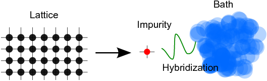
General reminder: Anderson impurity model and CTHYB solver

In the Anderson impurity model, we decompose the full lattice problem into an interacting site (‘impurity’) hybridised to a bath:

with the Hamiltonian :nbsphinx-math:`begin{align*}

H = & color{red}{H_{rm imp}} + color{darkgreen}{H_{rm hyb}} + color{blue}{H_{rm bath}} \ color{red}{H_{rm imp}} = & sum_{alpha beta} epsilon_{alpha beta} c^{dagger}_{alpha} c_{beta} + sum_{alpha beta gamma delta} U_{alpha beta gamma delta} c^{dagger}_{alpha} c^{dagger}_{beta} c_{delta} c_{gamma} \ color{darkgreen}{H_{rm hyb}} = & sum_{alpha nu k} (V_{alpha nu k} c^{dagger}_{alpha} d_{nu k} + h.~c.) \ color{blue}{H_{rm bath}} = & sum_{nu k} epsilon_{nu k} d^{dagger}_{nu k} d_{nu k}.

end{align*}`

The basic idea behind the CTHYB algorithm is to solve the impurity model by diagrammatically expanding the partition function \(Z\) in orders of the hybridization function. The resulting diagrams are then sampled stochastically using Monte Carlo while measuring quantities of interest, such as the Green’s function. Contrary to the IPT solver, CTHYB yields, within statistical error-bars, the exact solution of the impurity model.

The CTHYB solver needs two pieces of information as input from the user: - the interacting Hamiltonian, \(H_{\rm int} = \sum_{\alpha \beta \gamma \delta} U_{\alpha \beta \gamma \delta} c^{\dagger}_{\alpha} c^{\dagger}_{\beta} c_{\delta} c_{\gamma}\), - the non-interacting Green’s function, \(G_0(i\omega_n)\), from which the energy levels \(\epsilon\) and hybridization function are deduced.

The TRIQS/CTHYB impurity solver

In this notebook, we will see how to use the CTHYB impurity solver (documentation here). We will take the example of a single-orbital Anderson impurity model with a local Coulomb interaction on the impurity orbital

\[H_\mathrm{int} = U n_\mathrm{\uparrow} n_\mathrm{\downarrow}\]

The non-interacting Green’s function is

\[{\cal G}_0(i\omega_n) = \frac{1}{i\omega_n - \epsilon_d - V^2 \Gamma(i\omega_n)}\]

and \(\Gamma\) is the Green’s function of a flat conduction bath.

Setting up the impurity solver

Here is an example showing how to construct an impurity solver and run it on a single-orbital Anderson impurity model. Wait until the calculation is over before going on (see the “Kernel busy” solid circle on the top right).

from triqs.gfs import *
from triqs.operators import *
from triqs_cthyb import Solver

V = 1.0           # Hybridization strength
U = 4.0           # Local (on-site) Coulomb interaction
epsilon_d = 0.2   # Orbital energy level
beta = 20         # Inverse temperature

# Construct the impurity solver
S = Solver(beta = beta, gf_struct = [('up',1), ('down',1)] )

# Define the non-interacting Green's function
S.G0_iw << inverse(iOmega_n - epsilon_d - V**2 * Flat(1.0))

# Define the interacting Hamiltonian
h_int = U * n('up',0) * n('down',0)

# Solve the impurity problem for a given local Hamiltonian.
S.solve(h_int = h_int,
        length_cycle = 10,         # Number of steps between each measurement
        n_warmup_cycles = 5000,    # Number of warmup cycles
        n_cycles = 50000           # Number of QMC cycles
       )

Warning: could not identify MPI environment!

╔╦╗╦═╗╦╔═╗ ╔═╗  ┌─┐┌┬┐┬ ┬┬ ┬┌┐
 ║ ╠╦╝║║═╬╗╚═╗  │   │ ├─┤└┬┘├┴┐
 ╩ ╩╚═╩╚═╝╚╚═╝  └─┘ ┴ ┴ ┴ ┴ └─┘

The local Hamiltonian of the problem:

Starting serial run at: 2026-06-28 08:03:58.317947

0.2*c_dag('down',0)*c('down',0) + 0.2*c_dag('up',0)*c('up',0) + 4*c_dag('down',0)*c_dag('up',0)*c('up',0)*c('down',0)
Using autopartition algorithm to partition the local Hilbert space
Found 4 subspaces.
[Rank 0] Performing warmup phase...
[Rank 0] 08:03:58 100.00% done, ETA 00:00:00, cycle 5000 of 5000, 6.22e+04 cycles/sec
[Rank 0] Performing accumulation phase...
[Rank 0] 08:03:58  11.73% done, ETA 00:00:00, cycle 5867 of 50000, 5.87e+04 cycles/sec
[Rank 0] 08:03:59 100.00% done, ETA 00:00:00, cycle 50000 of 50000, 5.93e+04 cycles/sec
[Rank 0] Collect results: Waiting for all MPI processes to finish accumulating...

[Rank 0] Warmup duration: 0.0804 seconds [00:00:00]
[Rank 0] Simulation duration: 0.8438 seconds [00:00:00]
[Rank 0] Number of measures: 50000
[Rank 0] Cycles (measures) / second: 5.93e+04
[Rank 0] Measurement durations (total = 0.0281):
[Rank 0]   Measure Auto-correlation time: Duration = 0.0042
[Rank 0]   Measure Average order: Duration = 0.0012
[Rank 0]   Measure Average sign: Duration = 0.0011
[Rank 0]   Measure G_tau measure: Duration = 0.0216
[Rank 0] Move durations (total = 0.7844):
[Rank 0]   Move set Insert two operators: Duration = 0.1042
[Rank 0]     Move Insert Delta_up: Duration = 0.0482
[Rank 0]     Move Insert Delta_down: Duration = 0.0480
[Rank 0]   Move set Remove two operators: Duration = 0.0950
[Rank 0]     Move Remove Delta_up: Duration = 0.0435
[Rank 0]     Move Remove Delta_down: Duration = 0.0434
[Rank 0]   Move set Insert four operators: Duration = 0.1533
[Rank 0]     Move Insert Delta_up_up: Duration = 0.0410
[Rank 0]     Move Insert Delta_up_down: Duration = 0.0312
[Rank 0]     Move Insert Delta_down_up: Duration = 0.0315
[Rank 0]     Move Insert Delta_down_down: Duration = 0.0410
[Rank 0]   Move set Remove four operators: Duration = 0.1081
[Rank 0]     Move Remove Delta_up_up: Duration = 0.0226
[Rank 0]     Move Remove Delta_up_down: Duration = 0.0270
[Rank 0]     Move Remove Delta_down_up: Duration = 0.0269
[Rank 0]     Move Remove Delta_down_down: Duration = 0.0229
[Rank 0]   Move Shift one operator: Duration = 0.3238
[Rank 0] Move statistics:
[Rank 0]   Move set Insert two operators: Proposed = 99742, Accepted = 5108, Rate = 0.0512
[Rank 0]     Move Insert Delta_up: Proposed = 50040, Accepted = 2568, Rate = 0.0513
[Rank 0]     Move Insert Delta_down: Proposed = 49702, Accepted = 2540, Rate = 0.0511
[Rank 0]   Move set Remove two operators: Proposed = 99788, Accepted = 5089, Rate = 0.0510
[Rank 0]     Move Remove Delta_up: Proposed = 49992, Accepted = 2565, Rate = 0.0513
[Rank 0]     Move Remove Delta_down: Proposed = 49796, Accepted = 2524, Rate = 0.0507
[Rank 0]   Move set Insert four operators: Proposed = 99983, Accepted = 488, Rate = 0.0049
[Rank 0]     Move Insert Delta_up_up: Proposed = 25225, Accepted = 142, Rate = 0.0056
[Rank 0]     Move Insert Delta_up_down: Proposed = 24751, Accepted = 83, Rate = 0.0034
[Rank 0]     Move Insert Delta_down_up: Proposed = 24896, Accepted = 93, Rate = 0.0037
[Rank 0]     Move Insert Delta_down_down: Proposed = 25111, Accepted = 170, Rate = 0.0068
[Rank 0]   Move set Remove four operators: Proposed = 99948, Accepted = 496, Rate = 0.0050
[Rank 0]     Move Remove Delta_up_up: Proposed = 24672, Accepted = 142, Rate = 0.0058
[Rank 0]     Move Remove Delta_up_down: Proposed = 25150, Accepted = 96, Rate = 0.0038
[Rank 0]     Move Remove Delta_down_up: Proposed = 25058, Accepted = 87, Rate = 0.0035
[Rank 0]     Move Remove Delta_down_down: Proposed = 25068, Accepted = 171, Rate = 0.0068
[Rank 0]   Move Shift one operator: Proposed = 100539, Accepted = 69294, Rate = 0.6892

Total number of measures: 50000
Total cycles (measures) / second: 5.93e+04
Average sign: 1
Average order: 14.716
Auto-correlation time: 67.8791 cycles

Let’s try to explain the different lines of the script above. To construct the solver all that is needed is the inverse temperature \(\beta\) and a list that describes the block structure of the Green’s function. This is the gf_struct keyword. In this specific case, there are two (disconnected) blocks up and down and each containing only one orbital with the index 0. This is what is described by gf_struct.

In the next step, the member S.G0_iw of the solver is initialized. This Green’s function will be used as the non-interacting Green’s function when the solver starts.

The final step is to run the solver with the solve method. It has a certain number of parameters:

• h_int: This is the interacting Hamiltonian (i.e. the quartic terms in the local Hamiltonian, those with 4 operators) solved for in the Monte Carlo. It is defined using the operators that we have seen in the previous notebook. Important: the name of the indices in the operators have to be compatible with the gf_struct that was used in the construction of the solver.

• length_cycle: This is the number of steps at which measurements, e.g. of G_tau, are made to ensure data is decorrelated.

• n_warmup_cycles: The number of cycles used to thermalize the system.

• n_cycles: This is the number of Monte Carlo cycles, which is also the number of measures of the Green’s function.

For a more detailed discussion of TRIQS/CTHYB parameters please read our parameters guide.

Each calculation will have a Markov chain of length length_cycle * (n_warmup_cycles + n_cycles).

When the run is over, the outputs of the solver are:

• S.G_tau: The Green’s function in imaginary time of the system.

• S.G_iw: The Green’s function in Matsubara frequency of the system.

• S.Sigma_iw: The self-energy in Matsubara frequency.

Tips for advanced use: - For some more complex standard Hamiltonians, the library provides functions that can be used to construct h_int. See the operators section of the TRIQS documentation. - It is likely that for more involved calculations, you will have more parameters that you can adjust. See the online CTHYB documentation. - If you have many more parameters, it can be beneficial to set the parameters in a dictionary at the top of your script and simply pass the dictionary to solve using Python keyword arguments:

p = {}                        # Initialize an empty Python dictionary
p['length_cycle'] = 10        # Fill the dictionary with parameters
p['n_warmup_cycles'] = 5000
p['n_cycles'] = 50000

S.solve(h_int = h_int, **p)   # The dictionary contents will be unrolled as arguments to the solve function

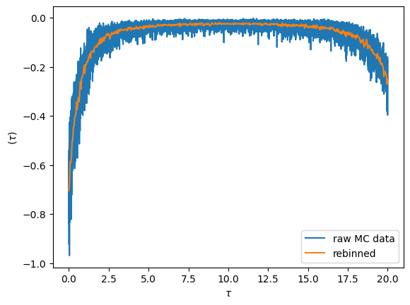
Visualizing the imaginary time sampled \(G(\tau)\)

Fundamentally the cthyb solver samples diagrams of the partition function. The imaginary time impurity Green’s function is then measured by removing individual hybridization lines, yielding samples at randomly chosen time-points. The samples at then gathered into bins obtained by splitting the interval \([0,\beta)\) into n_tau pieces.

We can visualize the result by plotting the raw data. The noise for each bin is inversely proportional the number of samples that fall into it. By increasing the bin-size we can reduce the noise level (but we introduce a systematic binning error). This is achieved with the rebinning_tau function

from triqs.plot.mpl_interface import *

oplot(S.G_tau['up'].real, '-', c='C0', label='raw MC data')

G_imp_rebinned = S.G_tau['up'].rebinning_tau(new_n_tau=500)
oplot(G_imp_rebinned.real, '-', c='C1', label='rebinned')

plt.legend(loc='lower right')
plt.show()

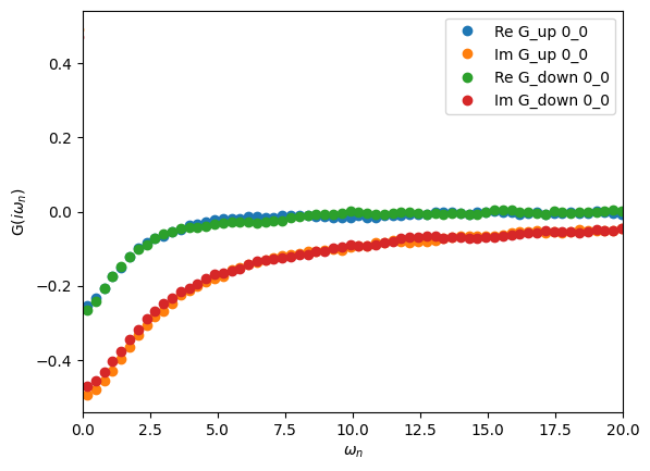
Visualizing the Matsubara-frequency results

We can also plot the results on the Matsubara axis and see how our statistics look in terms of the resulting noise. The solver automatically Fourier transforms S.G_tau to the Matsubara axis after finishing sampling, and the resulting Green’s function can be accessed as S.G_iw:

oplot(S.G_iw, 'o')
plt.xlim(0,20)
plt.show()

oplot(S.Sigma_iw, '-o')
plt.xlim(0,20)
plt.ylim(-1.0,2.0)
plt.show()

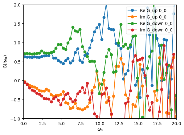
The large oscillations in the self-energy are due to a bad statistics in the Monte Carlo.

Exercise

---

Increase and decrease the number of Monte Carlo cycles to see its effect on the quality of the self-energy.