TRIQS Green’s functions
It is now time to start using some of the tools provided by TRIQS.
Much of the functionality in TRIQS, while implemented in C++ for optimal performance, is exposed through a Python interface to make it easier to use. In practice, this means you can treat TRIQS as a Python library, just like NumPy or matplotlib.
One of the central objects of a many-body calculation is a Green’s function. Green’s functions in TRIQS are functions defined on a mesh \(\cal{M}\) of points that hold values in some domain \(\cal{D}\), for example \(\mathbb{C}^{2\times2}\)
A few common Green’s function meshes in TRIQS include:
MeshReFreq- Real-frequencies equally spaced in \([\omega_{min},\omega_{max}]\)MeshImFreq- Matsubara FrequenciesMeshImTime- Imaginary time points equally spaced in \([0,\beta]\)MeshReTime- Real-time points (not covered in this tutorial)
Let’s see how we can construct a Mesh and print its values.
[1]:
# Import the Mesh type we want to use
from triqs.gfs import MeshImTime

# The documentation tells us which parameters we need to pass for the mesh construction
?MeshImTime
Python Library Documentation: class MeshImTime in module triqs.mesh.meshes

class MeshImTime(builtins.object)
 |  Imaginary time mesh type.
 |
 |  An imaginary time mesh is defined by its size :math:`N \geq 0`, an inverse temperature :math:`\beta > 0`
 |  and its particle statistics. It contains :math:`N` equally spaced mesh points on the interval :math:`[0, \beta]`
 |  such that the distance between two consecutive mesh points (step size) is constant.
 |
 |  An imaginary time mesh has the following properties:
 |
 |  - Each mesh point is identified by a unique index :math:`n \in \{0, 1, \ldots, N-1\}`.
 |  - An index :math:`n` is mapped to the corresponding data index :math:`d` by the identity function :math:`d(n) = n`
 |    and vice versa.
 |  - An index :math:`n` is mapped to the corresponding value :math:`\tau` by the linear function
 |    :math:`\tau(n) = n \cdot \Delta` such that :math:`\tau(0) = 0` and :math:`\tau(N-1) = \beta`. The step size of
 |    the mesh is :math:`\Delta = \frac{\beta}{N - 1}` for :math:`N > 1`, otherwise it is undefined. For implementation
 |    purposes, we set :math:`\Delta = 0` and :math:`\Delta^{-1} = 0` for :math:`N = 0` and :math:`\Delta = 0` and
 |    :math:`\Delta^{-1} = \infty` for :math:`N = 1`.
 |  - An arbitrary value :math:`\tau \in [0, \beta]` is mapped to the closest mesh point with index :math:`n` by the
 |    function :math:`n(\tau) = \left\lfloor \frac{\tau}{\Delta} + 0.5 \right\rfloor`.
 |
 |  Green's function containers that are based on an imaginary time mesh store the function values at the discrete time
 |  points :math:`\tau(n)`, i.e. :math:`f_n = f(\tau(n))`, and use linear interpolation to evaluate the function at an
 |  arbitrary imaginary time :math:`\tau \in [0, \beta]`.
 |
 |  ----------
 |
 |  Dispatched C++ constructor(s).
 |
 |  ::
 |
 |     [1] (beta: float = 1, statistic: Statistic ("Fermion" | "Boson") = 1, n_tau: int = 0)
 |
 |
 |  Construct an imaginary time mesh on the interval :math:`[0, \beta]` with :math:`N \geq 0` equally spaced
 |  mesh points and the given particle statistics.
 |
 |  Parameters
 |  ----------
 |  beta : float
 |     Inverse temperature :math:`\beta > 0`.
 |  statistic : Statistic ("Fermion" | "Boson")
 |     Particle statistics.
 |  n_tau : int
 |     Size of the mesh.
 |
 |  Methods defined here:
 |
 |  __call__(self, /, *args, **kwargs)
 |      Call self as a function.
 |
 |  __eq__(self, value, /)
 |      Return self==value.
 |
 |  __ge__(self, value, /)
 |      Return self>=value.
 |
 |  __getitem__(self, key, /)
 |      Return self[key].
 |
 |  __getstate__(...)
 |      Helper for pickle.
 |
 |  __gt__(self, value, /)
 |      Return self>value.
 |
 |  __init__(self, /, *args, **kwargs)
 |      Initialize self.  See help(type(self)) for accurate signature.
 |
 |  __iter__(self, /)
 |      Implement iter(self).
 |
 |  __le__(self, value, /)
 |      Return self<=value.
 |
 |  __len__(self, /)
 |      Return len(self).
 |
 |  __lt__(self, value, /)
 |      Return self<value.
 |
 |  __ne__(self, value, /)
 |      Return self!=value.
 |
 |  __repr__(self, /)
 |      Return repr(self).
 |
 |  __setstate__(...)
 |
 |  __str__(self, /)
 |      Return str(self).
 |
 |  __write_hdf5__(...)
 |
 |  copy(...)
 |      Dispatched C++ function(s).
 |
 |      ::
 |
 |         [1] ()
 |           -> MeshImTime
 |
 |
 |      Get a copy of a mesh (for Python bindings).
 |
 |      Parameters
 |      ----------
 |      m : MeshImTime
 |         The mesh object to copy.
 |
 |      Returns
 |      -------
 |      MeshImTime
 |         Copy of the given mesh.
 |
 |  copy_from(...)
 |      Dispatched C++ function(s).
 |
 |      ::
 |
 |         [1] (m2: MeshImTime)
 |           -> void
 |
 |
 |      Copy one mesh into another (for Python bindings).
 |
 |      Simply calls the copy assignment operator of the mesh.
 |
 |      Parameters
 |      ----------
 |      m1 : MeshImTime
 |         The mesh object to copy into.
 |      m2 : MeshImTime
 |         The mesh object to copy from.
 |
 |  is_index_valid(...)
 |      Dispatched C++ function(s).
 |
 |      ::
 |
 |         [1] (n: int)
 |           -> bool
 |
 |
 |      Check if an index :math:`n` is valid.
 |
 |      Parameters
 |      ----------
 |      n : int
 |         Index :math:`n` to check.
 |
 |      Returns
 |      -------
 |      bool
 |         True if :math:`0 \leq n < N`, false otherwise.
 |
 |  to_data_index(...)
 |      Dispatched C++ function(s).
 |
 |      ::
 |
 |         [1] (n: int)
 |           -> int
 |
 |
 |      Map an index :math:`n \in \{0, 1, \ldots, N-1\}` to its corresponding data index :math:`d(n)`.
 |
 |      Parameters
 |      ----------
 |      n : int
 |         Index :math:`n` to map.
 |
 |      Returns
 |      -------
 |      int
 |         Data index :math:`d(n) = n`.
 |
 |  to_index(...)
 |      Dispatched C++ function(s).
 |
 |      ::
 |
 |         [1] (d: int)
 |           -> int
 |
 |
 |      Map a data index :math:`d \in \{0, 1, \ldots, N-1\}` to the corresponding index :math:`n(d)`.
 |
 |      Parameters
 |      ----------
 |      d : int
 |         Data index :math:`d` to map.
 |
 |      Returns
 |      -------
 |      int
 |         Index :math:`n(d) = d`.
 |
 |  to_value(...)
 |      Dispatched C++ function(s).
 |
 |      ::
 |
 |         [1] (n: int)
 |           -> float
 |
 |
 |      Map an index :math:`n \in \{0, 1, \ldots, N-1\}` to its corresponding value :math:`m(n)`.
 |
 |      Parameters
 |      ----------
 |      n : int
 |         Index :math:`n` to map.
 |
 |      Returns
 |      -------
 |      float
 |         Value of the mesh point :math:`m(n) = a + n \cdot \Delta`.
 |
 |  values(...)
 |      Dispatched C++ function(s).
 |
 |      ::
 |
 |         [1] ()
 |           -> ndarray[float, 1]
 |
 |
 |      Get the values of all mesh points in a mesh.
 |
 |      Parameters
 |      ----------
 |      m : MeshImTime
 |         A mesh object.
 |
 |      Returns
 |      -------
 |      ndarray[float, 1]
 |         Array containing the values of all mesh points.
 |
 |  ----------------------------------------------------------------------
 |  Static methods defined here:
 |
 |  __new__(*args, **kwargs)
 |      Create and return a new object.  See help(type) for accurate signature.
 |
 |  ----------------------------------------------------------------------
 |  Data descriptors defined here:
 |
 |  beta
 |      Get the inverse temperature :math:`\beta`.
 |
 |  delta
 |      Get the step size :math:`\Delta` of the mesh, i.e. the distance between two consecutive mesh points.
 |
 |  delta_inv
 |      Get the inverse of the step size of the mesh, i.e. :math:`1 / \Delta`.
 |
 |  first_index
 |      Get the first index of the mesh, i.e. :math:`0`.
 |
 |  last_index
 |      Get the last index of the mesh, i.e. :math:`N - 1`.
 |
 |  mesh_hash
 |      Get the hash value of the mesh.
 |
 |  statistic
 |      Get the particle statistics.
 |
 |  ----------------------------------------------------------------------
 |  Data and other attributes defined here:
 |
 |  __hash__ = None
[2]:
# Provide the inverse temperature, Statistic, and number of points
tau_mesh = MeshImTime(beta=5, statistic='Fermion', n_tau=11)

# We can loop and print the mesh-point values
for tau in tau_mesh:
    print(tau.value)

    # Using tab for auto completion can be very helpful to understand
    # which other members, functions and properties are available for
    # a given Python object like 'tau'.
    # Type 'tau.' below and use tab to see which options you get!
0.0
0.5
1.0
1.5
2.0
2.5
3.0
3.5
4.0
4.5
5.0
Now let’s create and initialize a Green’s function for a single atomic level with energy \(\epsilon\) in the grand-canonical ensemble with inverse temperature \(\beta\)
We first have a look at the documentation for Gf.
[3]:
from triqs.gfs import Gf
?Gf
Python Library Documentation: class Gf in module triqs.gfs.gf
class Gf(builtins.object)
| Gf(**kw)
|
| Container for Green's functions and related quantities.
|
| A :class:`~triqs.gfs.gf.Gf` is a container for generic functions defined on
| meshes:
|
| .. math::
|
| G : \mathcal{M} \to T .
|
| Here, :math:`\mathcal{M}` is the domain of the function, determined
| entirely by the underlying mesh (see :mod:`triqs.mesh.meshes`) or
| :class:`~triqs.mesh.mesh_product.MeshProduct`, and :math:`T` is the
| target space, which determines what quantities are stored at each
| mesh point (real/complex scalars, matrices, tensors).
|
| Typical use cases include
|
| - scalar-valued imaginary time Green's functions
|
| .. math::
|
| G(\tau) \equiv - \mathcal{T} \langle c(\tau) c^{\dagger} (0)\rangle
| \qquad \text{ for } 0 \leq \tau \leq \beta \; ,
|
| with :class:`~triqs.mesh.meshes.MeshImTime` as the underlying mesh
| and :math:`T = \mathbb{R}` as the target space.
| - matrix-valued Matsubara Green's functions
|
| .. math::
|
| G_{\alpha \beta} (i \omega_n) \equiv \int_0^\beta
| G_{\alpha \beta}(\tau) e^{i \omega_n \tau} d\tau \; ,
|
| with :class:`~triqs.mesh.meshes.MeshImFreq` as the underlying mesh
| and :math:`T = \mathbb{C}^{N \times N}` as the target space.
|
| Under the hood, :class:`~triqs.gfs.gf.Gf` stores a contiguous ``numpy.ndarray`` of
| shape ``(*mesh_sizes, *target_shape)`` (see :attr:`~triqs.gfs.gf.Gf.data`). What is
| stored and how Green's functions are evaluated depends on the mesh.
|
| Supported features include:
|
| - Bracket lookup ``g[...]`` and call-style evaluation ``g(...)``
| (see Notes).
| - Element-wise arithmetic (``+``, ``-``, ``*``, ``/``, ``@``) and
| in-place variants. Scalars broadcast along the target-space
| diagonal for square matrix targets; mixing two :class:`~triqs.gfs.gf.Gf`
| requires identical meshes.
| - Lazy initialization via ``g << expr`` from descriptors
| (e.g. ``g << iOmega_n + 0.5``, ``g << SemiCircular(1.0)``).
| See :meth:`~triqs.gfs.gf.Gf.__lshift__` and :mod:`triqs.gfs.descriptors`.
| - HDF5 read/write through :class:`h5.HDFArchive`.
| - Target-space slicing and :attr:`~triqs.gfs.gf.Gf.real` / :attr:`~triqs.gfs.gf.Gf.imag` views.
|
| Parameters
| ----------
| mesh : Mesh or MeshProduct
| Mesh on which the Green's function is defined.
| data : numpy.ndarray, optional
| Raw storage of shape ``(*mesh_sizes, *target_shape)``. Mutually
| exclusive with :attr:`~triqs.gfs.gf.Gf.target_shape`.
| target_shape : list of int, optional
| Shape of the target space (e.g. ``[2, 2]`` for a 2x2 matrix
| Green's function, ``[]`` for a scalar). Mutually exclusive with
| :attr:`~triqs.gfs.gf.Gf.data`.
| is_real : bool, optional
| If ``True`` (and :attr:`~triqs.gfs.gf.Gf.target_shape` is given), allocate the data
| as ``float64`` instead of ``complex128``. Has no effect when
| :attr:`~triqs.gfs.gf.Gf.data` is supplied. Default ``False``.
| name : str, optional
| Name used for plot labels. Default ``''``.
| indices : list, optional
| Deprecated. String indices are no longer supported; passing this
| argument emits a :class:`FutureWarning` and the lengths are used
| to derive :attr:`~triqs.gfs.gf.Gf.target_shape`.
|
| Attributes
| ----------
| mesh : Mesh
| The mesh of the Green's function.
| data : numpy.ndarray
| Raw data, shape ``(*mesh_sizes, *target_shape)``.
| rank : int
| Number of mesh axes (``mesh.rank``).
| target_rank : int
| Number of target-space axes (``len(target_shape)``).
| target_shape : tuple of int
| Shape of the target space.
| name : str
| Plot label.
| real : Gf
| Views of the real part of the :attr:`~triqs.gfs.gf.Gf.data`.
| imag : Gf
| Views of imaginary real part of the :attr:`~triqs.gfs.gf.Gf.data`.
|
| Notes
| -----
| There are subtle differences when accessing a :class:`~triqs.gfs.gf.Gf` with brackets
| ``[]`` vs. parentheses ``()``:
|
| - ``g[x]`` looks up the value at an *existing* mesh point, with ``x``
| an :class:`~triqs.gfs.gf.Idx`, :class:`~triqs.mesh.mesh_point.MeshPoint`, or
| :class:`~triqs.mesh.matsubara_freq.MatsubaraFreq`.
| - ``g(x)`` instead *evaluates* the Green's function at an arbitrary ``x``
| using the interpolation rule the mesh declares -- linear in imaginary time,
| exact in Matsubara, k-linear on the Brillouin zone, basis expansion on
| DLR / Legendre, etc. The mesh, not the :class:`~triqs.gfs.gf.Gf`, decides what
| "evaluation" means.
|
| Examples
| --------
| Construct a scalar imaginary-time Green's function and a 2x2
| matrix-valued Matsubara Green's function:
|
| >>> from triqs.gfs import Gf
| >>> from triqs.mesh import MeshImTime, MeshImFreq
| >>> tau_mesh = MeshImTime(beta=10.0, statistic='Fermion', n_tau=2049)
| >>> g_tau = Gf(mesh=tau_mesh, target_shape=[])
| >>> iw_mesh = MeshImFreq(beta=10.0, statistic='Fermion', n_iw=1024)
| >>> g_iw = Gf(mesh=iw_mesh, target_shape=[2, 2])
|
| Initialize lazily from a descriptor expression:
|
| >>> from triqs.gfs import iOmega_n, SemiCircular
| >>> g_iw << iOmega_n + 0.5
| >>> g_tau << SemiCircular(half_bandwidth=1.0)
|
| Access the raw storage as a numpy array:
|
| >>> g_iw.data.shape
| (2048, 2, 2)
| >>> g_iw.data[:] = 0.0 # zero in place
|
| Methods defined here:
|
| __add__(self, y)
| Element-wise addition; returns a new :class:`~triqs.gfs.gf.Gf`.
|
| Parameters
| ----------
| y : Gf, descriptor, lazy expression, scalar or numpy.ndarray
| Right-hand operand.
|
| Returns
| -------
| Gf or LazyExpr
| ``self + y`` as a fresh object.
|
| __call__(self, *args)
| Evaluate the Green's function at the given point(s).
|
| Parameters
| ----------
| *args
| One value per mesh axis. Each value may be a raw scalar
| (e.g. a complex frequency, a real frequency, an imaginary
| time, ...), a :class:`~triqs.mesh.mesh_point.MeshPoint` or an
| :class:`~triqs.gfs.gf.Idx`.
|
| Returns
| -------
| numpy.ndarray
| Value of the Green's function at the requested point, of
| shape ``target_shape``. Interpolation between mesh points is
| applied where supported by the C++ backend.
|
| Notes
| -----
| Dispatches to a C++ ``CallProxy*`` selected from the mesh and
| target rank. For mesh / target combinations without a proxy this
| method raises :class:`NotImplementedError`.
|
| __getitem__(self, key)
| Return a mesh point, a sliced view, or a target-space sub-block.
|
| The bracket operator dispatches on the type of ``key``:
|
| * ``g[:]`` — return ``self`` (so that ``g[:] << RHS`` is
| equivalent to ``g << RHS``).
| * ``g[mp]`` with ``mp`` a :class:`~triqs.mesh.mesh_point.MeshPoint`,
| :class:`~triqs.gfs.gf.Idx` or :class:`~triqs.mesh.matsubara_freq.MatsubaraFreq` —
| return the target-space slab at that mesh point (a numpy array).
| * ``g[mp0, mp1, ...]`` — same, for a :class:`~triqs.mesh.mesh_product.MeshProduct`.
| * ``g[mp, :]`` (mix of mesh points and ``:``) — return a
| :class:`~triqs.gfs.gf.Gf` on the remaining mesh axes.
| * ``g[i, j, ...]`` with all-integer indices — extract a
| ``target_rank``-dimensional sub-block as a :class:`~triqs.gfs.gf.Gf` view of
| reduced target rank.
| * ``g[i:j, ...]`` with all-slice indices — slice the target
| space and return a :class:`~triqs.gfs.gf.Gf` view.
|
| Parameters
| ----------
| key : slice, MeshPoint, Idx, MatsubaraFreq, int, or tuple thereof
| See the bullet list above.
|
| Returns
| -------
| Gf or numpy.ndarray
| A :class:`~triqs.gfs.gf.Gf` view when the operation slices the mesh or
| target space; a numpy array when ``key`` resolves to a
| single mesh point.
|
| Notes
| -----
| Partial slicing of the mesh and string indices are not
| supported.
|
| __iadd__(self, arg)
| In-place addition ``self += arg`` (element-wise on ``self.data``).
|
| Parameters
| ----------
| arg : Gf, descriptor, lazy expression, scalar or numpy.ndarray
| Operand. A scalar added to a matrix-valued Gf is broadcast
| along the diagonal of the target space.
|
| Returns
| -------
| Gf or LazyExpr
| ``self`` (or a lazy expression if ``arg`` is lazy).
|
| __imatmul__(self, arg)
| In-place matrix multiplication ``self @= arg`` on the target space.
|
| Evaluated pointwise on the mesh. Rank-0 (scalar-valued) and
| rank-2 (matrix-valued) Green's functions are supported; mixed
| ``rank-0 * rank-2`` broadcasts the scalar value across the
| target-space matrix.
|
| Parameters
| ----------
| arg : Gf, lazy expression, scalar or numpy.ndarray
| Right-hand operand.
|
| Returns
| -------
| Gf or LazyExpr
|
| __imul__(self, arg)
| In-place multiplication ``self *= arg`` (alias for :meth:`~triqs.gfs.gf.Gf.__imatmul__`).
|
| Parameters
| ----------
| arg : Gf, scalar or numpy.ndarray
|
| Returns
| -------
| Gf
|
| __init__(self, **kw)
| Initialize self. See help(type(self)) for accurate signature.
|
| __isub__(self, arg)
| In-place subtraction ``self -= arg``.
|
| Parameters
| ----------
| arg : Gf, descriptor, lazy expression, scalar or numpy.ndarray
| Operand.
|
| Returns
| -------
| Gf or LazyExpr
|
| __itruediv__(self, arg)
| In-place scalar division ``self /= arg``.
|
| Parameters
| ----------
| arg : scalar
| Divisor applied element-wise to ``self.data``.
|
| Returns
| -------
| Gf
|
| __lazy_expr_eval_context__(self)
|
| __le__(self, other)
| Return self<=value.
|
| __lshift__(self, A)
| Lazy initialization / copy operator (``g << RHS``).
|
| Parameters
| ----------
| A : Gf, descriptor or :class:`~triqs.gfs.lazy_expressions.LazyExpr`
| * If ``A`` is a :class:`~triqs.gfs.gf.Gf` on the same mesh, copy it into
| ``self``.
| * If ``A`` is a descriptor (e.g. :class:`~triqs.gfs.descriptors.SemiCircular`,
| :class:`~triqs.gfs.descriptors.Flat`, :data:`~triqs.gfs.descriptor_base.iOmega_n`)
| or a lazy expression built from descriptors and scalars, evaluate it on
| ``self.mesh`` and store the result.
| * If ``A`` is a scalar, fill the diagonal of the target
| space with that scalar.
|
| Returns
| -------
| Gf
| ``self`` (so that ``g << RHS`` can be chained).
|
| Examples
| --------
| >>> g << iOmega_n + 0.5
| >>> g << SemiCircular(half_bandwidth=1.0)
| >>> g2 << g
|
| __matmul__(self, y)
| Matrix multiplication ``self @ y`` on the target space.
|
| For Matsubara meshes the result mesh statistic follows the
| bosonic / fermionic combination rule of the operands.
|
| Parameters
| ----------
| y : Gf, scalar or numpy.ndarray
| Right-hand operand.
|
| Returns
| -------
| Gf
| Product evaluated pointwise on the mesh; freshly allocated.
|
| __mul__(self, y)
| Multiplication ``self * y`` (alias for :meth:`~triqs.gfs.gf.Gf.__matmul__`).
|
| For matrix-valued Green's functions this is the target-space
| matrix product evaluated pointwise on the mesh.
|
| Parameters
| ----------
| y : Gf, scalar or numpy.ndarray
|
| Returns
| -------
| Gf
|
| __neg__(self)
| Unary minus ``-self``; returns a new :class:`~triqs.gfs.gf.Gf` with sign-flipped data.
|
| Returns
| -------
| Gf
|
| __radd__(self, y)
| Reflected addition ``y + self``; commutes with :meth:`~triqs.gfs.gf.Gf.__add__`.
|
| Parameters
| ----------
| y : same as :meth:`~triqs.gfs.gf.Gf.__add__`
|
| Returns
| -------
| Gf or LazyExpr
|
| __reduce__(self)
| Helper for pickle.
|
| __reduce_to_dict__(self)
|
| __repr__(self)
| One-line summary of the Green's function.
|
| Returns
| -------
| str
| ``"Green's Function <name> with mesh <mesh> and target_shape <target_shape>"``.
|
| __rmatmul__(self, y)
| Reflected matrix multiplication ``y @ self``.
|
| Parameters
| ----------
| y : scalar or 2D numpy.ndarray
| Left-hand operand.
|
| Returns
| -------
| Gf
|
| __rmul__(self, y)
| Reflected multiplication ``y * self``.
|
| Parameters
| ----------
| y : scalar or numpy.ndarray
|
| Returns
| -------
| Gf
|
| __rsub__(self, y)
| Reflected subtraction ``y - self``.
|
| Parameters
| ----------
| y : same as :meth:`~triqs.gfs.gf.Gf.__sub__`
|
| Returns
| -------
| Gf or LazyExpr
|
| __setitem__(self, key, val)
| Assign at a mesh point or delegate to ``<<`` for everything else.
|
| ``g[mp] = val`` writes ``val`` into ``self.data`` at the data
| index corresponding to ``mp`` (a :class:`~triqs.mesh.mesh_point.MeshPoint`,
| :class:`~triqs.gfs.gf.Idx` or :class:`~triqs.mesh.matsubara_freq.MatsubaraFreq`,
| or a tuple of those for a :class:`~triqs.mesh.mesh_product.MeshProduct`). Any
| other shape of ``key`` falls back to ``self[key] << val``.
|
| Parameters
| ----------
| key : MeshPoint, Idx, MatsubaraFreq, tuple thereof
| Assignment target.
| val : array-like or Gf-compatible
| Value or Green's function to assign.
|
| __str__(self)
| Alias for :meth:`~triqs.gfs.gf.Gf.__repr__`.
|
| Returns
| -------
| str
|
| __sub__(self, y)
| Element-wise subtraction; returns a new :class:`~triqs.gfs.gf.Gf`.
|
| Parameters
| ----------
| y : same as :meth:`~triqs.gfs.gf.Gf.__isub__`
|
| Returns
| -------
| Gf or LazyExpr
| ``self - y``.
|
| __truediv__(self, y)
| Scalar division ``self / y``; returns a new :class:`~triqs.gfs.gf.Gf`.
|
| Parameters
| ----------
| y : scalar
| Divisor.
|
| Returns
| -------
| Gf
|
| conjugate(self)
| Conjugate of the Green's function.
|
| Returns
| -------
| G : Gf (copy)
| Conjugate of the Green's function.
|
| copy(self)
| Return an independent deep copy of ``self``.
|
| Returns
| -------
| Gf
| Copy with freshly allocated mesh and data arrays.
|
| copy_from(self, another)
| In-place copy from ``another`` into ``self``.
|
| Parameters
| ----------
| another : Gf
| Source Green's function. Must have an identical data shape;
| its mesh is copied into ``self.mesh``.
|
| Raises
| ------
| AssertionError
| If ``self.data.shape != another.data.shape``.
|
| density(self, *args, **kwargs)
| Compute the single-particle density matrix.
|
| Equivalent to :math:`\langle c^\dagger_i c_j \rangle` evaluated
| from the diagonal-frequency / equal-time limit of the Green's
| function.
|
| Parameters
| ----------
| beta : float, optional
| Inverse temperature. Required only for finite-temperature
| density evaluation on a :class:`~triqs.mesh.meshes.MeshReFreq` mesh.
|
| Returns
| -------
| density_matrix : numpy.ndarray
| Single-particle density matrix of shape ``target_shape``.
|
| Notes
| -----
| Only available for single-mesh Green's functions on a Matsubara,
| real-frequency or Legendre mesh.
|
| enforce_discontinuity(self, *args, **kw) from triqs.gfs.gf.add_method_helper.<locals>
| Dispatched C++ function(s).
|
| ::
|
| [1] (gl: Gf[MeshLegendre, 2], disc: ndarray[float, 2])
| -> void
|
|
| Enforce a prescribed jump at :math:`\tau = 0` for a Legendre Green's function.
|
| The Legendre coefficients are adjusted in place so that the corresponding imaginary-time Green's
| function has the specified discontinuity :math:`G(0^+) - G(0^-)` at :math:`\tau = 0` (which equals :math:`-1` for
| a fermionic propagator). Coefficients above the constrained subspace are left unchanged.
|
| Parameters
| ----------
| gl : Gf[MeshLegendre, 2]
| Legendre Green's function modified in place.
| disc : ndarray[float, 2]
| Target discontinuity at :math:`\tau = 0`.
|
| fit_hermitian_tail(self, *args, **kw) from triqs.gfs.gf.add_method_helper.<locals>
| Dispatched C++ function(s).
|
| ::
|
| [1] (g: Gf[MeshImFreq, 2],
| known_moments: ndarray[complex, 3] = [])
| -> tuple[ndarray[complex, 3], float]
|
| [2] (g: Gf[MeshImFreq, 0],
| known_moments: ndarray[complex, 1] = [])
| -> tuple[ndarray[complex, 1], float]
|
| [3] (bg: BlockGf[MeshImFreq, 2],
| known_moments: [ndarray[complex, 3]] = <unprintable>)
| -> tuple[[ndarray[complex, 3]], float]
|
| [4] (bg: BlockGf[MeshImFreq, 0],
| known_moments: [ndarray[complex, 1]] = <unprintable>)
| -> tuple[[ndarray[complex, 1]], float]
|
|
| [1, 2] Fit the high-frequency tail of a Green's function, imposing hermitian symmetry on the fitted moments.
|
| The symmetry constraint is :math:`G_{i,j}(i\omega) = G_{j,i}^*(-i\omega)`.
|
| ------
|
| [3, 4] Fit the high-frequency tail of a block Green's function, imposing hermitian symmetry block by block.
|
| The symmetry constraint is :math:`G_{i,j}(i\omega) = G_{j,i}^*(-i\omega)`.
|
| Each block is fitted independently with the same symmetry constraint. The returned error is the maximum across
| blocks.
|
| ------
|
| Parameters
| ----------
| g : Gf[MeshImFreq, 2], Gf[MeshImFreq, 0]
| The Green's function whose tail is to be fitted.
| known_moments : ndarray[complex, 3], ndarray[complex, 1]
| Array of known high-frequency moments to constrain the fit.
| bg : BlockGf[MeshImFreq, 2], BlockGf[MeshImFreq, 0]
| The block Green's function whose tail is to be fitted.
|
| Returns
| -------
| [1] : tuple[ndarray[complex, 3], float]
| A pair containing the fitted tail moments and the fitting error.
|
| [2] : tuple[ndarray[complex, 1], float]
| A pair containing the fitted tail moments and the fitting error.
|
| [3] : tuple[[ndarray[complex, 3]], float]
| A pair containing the per-block fitted tail moments and the worst-block fitting error.
|
| [4] : tuple[[ndarray[complex, 1]], float]
| A pair containing the per-block fitted tail moments and the worst-block fitting error.
|
| fit_hermitian_tail_on_window(self, *args, **kw) from triqs.gfs.gf.add_method_helper.<locals>
| Dispatched C++ function(s).
|
| ::
|
| [1] (g: Gf[MeshImFreq, 2],
| n_min: int,
| n_max: int,
| known_moments: ndarray[complex, 3],
| n_tail_max: int,
| expansion_order: int)
| -> tuple[ndarray[complex, 3], float]
|
|
| Fit the high-frequency tail on a restricted window, imposing hermitian moment matrices.
|
| Behaves like ``fit_tail_on_window`` but enforces the symmetry :math:`G_{i,j}(i\omega) =
| G_{j,i}^*(-i\omega)` on the fitted moments.
|
| Parameters
| ----------
| g : Gf[MeshImFreq, 2]
| The Matsubara Green's function whose tail is to be fitted.
| n_min : int
| Minimum Matsubara index of the fit window.
| n_max : int
| Maximum Matsubara index of the fit window (:math:`-1` means use the last index of the mesh).
| known_moments : ndarray[complex, 3]
| Array of known high-frequency moments to constrain the fit.
| n_tail_max : int
| Maximum frequency index used internally by the tail fitter.
| expansion_order : int
| Order of the tail expansion to fit.
|
| Returns
| -------
| tuple[ndarray[complex, 3], float]
| A pair containing the fitted tail moments and the fitting error.
|
| fit_tail(self, *args, **kw) from triqs.gfs.gf.add_method_helper.<locals>
| Dispatched C++ function(s).
|
| ::
|
| [1] (g: Gf[MeshImFreq, 2],
| known_moments: ndarray[complex, 3] = [])
| -> tuple[ndarray[complex, 3], float]
|
| [2] (g: Gf[MeshImFreq, 0],
| known_moments: ndarray[complex, 1] = [])
| -> tuple[ndarray[complex, 1], float]
|
| [3] (g: Gf[MeshReFreq, 2],
| known_moments: ndarray[complex, 3] = [])
| -> tuple[ndarray[complex, 3], float]
|
| [4] (g: Gf[MeshReFreq, 0],
| known_moments: ndarray[complex, 1] = [])
| -> tuple[ndarray[complex, 1], float]
|
| [5] (bg: BlockGf[MeshImFreq, 2],
| known_moments: [ndarray[complex, 3]] = <unprintable>)
| -> tuple[[ndarray[complex, 3]], float]
|
| [6] (bg: BlockGf[MeshImFreq, 0],
| known_moments: [ndarray[complex, 1]] = <unprintable>)
| -> tuple[[ndarray[complex, 1]], float]
|
| [7] (bg: BlockGf[MeshReFreq, 2],
| known_moments: [ndarray[complex, 3]] = <unprintable>)
| -> tuple[[ndarray[complex, 3]], float]
|
| [8] (bg: BlockGf[MeshReFreq, 0],
| known_moments: [ndarray[complex, 1]] = <unprintable>)
| -> tuple[[ndarray[complex, 1]], float]
|
|
| [1, 2, 3, 4] Fit the high-frequency tail of a Green's function using a least-squares procedure.
|
| The result is the set of expansion moments that best reproduces the high-frequency behavior of :math:`G`
| on the configured tail-fit window. Known moments, when provided, are treated as exact constraints on the fit.
|
| ------
|
| [5, 6, 7, 8] Fit the high-frequency tail of a block Green's function using a least-squares procedure.
|
| Each block is fitted independently using ``fit_tail``. The returned error is the maximum across blocks.
|
| ------
|
| Parameters
| ----------
| g : Gf[MeshImFreq, 2], Gf[MeshImFreq, 0], Gf[MeshReFreq, 2], Gf[MeshReFreq, 0]
| The Green's function whose tail is to be fitted.
| known_moments : ndarray[complex, 3], ndarray[complex, 1]
| Array of known high-frequency moments to constrain the fit.
| bg : BlockGf[MeshImFreq, 2], BlockGf[MeshImFreq, 0], BlockGf[MeshReFreq, 2], BlockGf[MeshReFreq, 0]
| The block Green's function whose tail is to be fitted.
|
| Returns
| -------
| [1, 3] : tuple[ndarray[complex, 3], float]
| A pair containing the fitted tail moments and the fitting error.
|
| [2, 4] : tuple[ndarray[complex, 1], float]
| A pair containing the fitted tail moments and the fitting error.
|
| [5, 7] : tuple[[ndarray[complex, 3]], float]
| A pair containing the per-block fitted tail moments and the worst-block fitting error.
|
| [6, 8] : tuple[[ndarray[complex, 1]], float]
| A pair containing the per-block fitted tail moments and the worst-block fitting error.
|
| fit_tail_on_window(self, *args, **kw) from triqs.gfs.gf.add_method_helper.<locals>
| Dispatched C++ function(s).
|
| ::
|
| [1] (g: Gf[MeshImFreq, 2],
| n_min: int,
| n_max: int,
| known_moments: ndarray[complex, 3],
| n_tail_max: int,
| expansion_order: int)
| -> tuple[ndarray[complex, 3], float]
|
|
| Fit the high-frequency tail of a Matsubara Green's function on a restricted frequency window.
|
| The fit is performed on the window :math:`[n_{\min}, n_{\max}]` of the Matsubara mesh (:math:`n_{\max} =
| -1` selects the last index of the mesh). The tail fitter is configured from ``n_tail_max`` and
| ``expansion_order``, and the fit is delegated to ``fit_tail``.
|
| Parameters
| ----------
| g : Gf[MeshImFreq, 2]
| The Matsubara Green's function whose tail is to be fitted.
| n_min : int
| Minimum Matsubara index of the fit window.
| n_max : int
| Maximum Matsubara index of the fit window (:math:`-1` means use the last index of the mesh).
| known_moments : ndarray[complex, 3]
| Array of known high-frequency moments to constrain the fit.
| n_tail_max : int
| Maximum frequency index used internally by the tail fitter.
| expansion_order : int
| Order of the tail expansion to fit.
|
| Returns
| -------
| tuple[ndarray[complex, 3], float]
| A pair containing the fitted tail moments and the fitting error.
|
| from_L_G_R(self, L, G, R)
| Matrix transform of the target space of a matrix valued Green's function.
|
| Sets the current Green's function :math:`g_{ab}` to the matrix transform of :math:`G_{cd}`
| using the left and right transform matrices :math:`L_{ac}` and :math:`R_{db}`.
|
| .. math::
| g_{ab} = \sum_{cd} L_{ac} G_{cd} R_{db}
|
| Parameters
| ----------
| L : (a, c) ndarray
| Left side transform matrix.
| G : Gf matrix valued target_shape == (c, d)
| Green's function to transform.
| R : (d, b) ndarray
| Right side transform matrix.
|
| Notes
| -----
| Only implemented for Green's functions with a single mesh.
|
| inverse(self)
| Computes the inverse of the Green's function.
|
| Returns
| -------
| G : Gf (copy)
| The matrix/scalar inverse of the Green's function.
|
| invert(self)
| Inverts the Green's function (in place).
|
| is_gf_hermitian(self, *args, **kw) from triqs.gfs.gf.add_method_helper.<locals>
| Dispatched C++ function(s).
|
| ::
|
| [1] (g: Gf[MeshImFreq, 0], tolerance: float = 1e-12)
| -> bool
|
| [2] (g: Gf[MeshImFreq, 2], tolerance: float = 1e-12)
| -> bool
|
| [3] (g: Gf[MeshImFreq, 4], tolerance: float = 1e-12)
| -> bool
|
| [4] (g: BlockGf[MeshImFreq, 0], tolerance: float = 1e-12)
| -> bool
|
| [5] (g: BlockGf[MeshImFreq, 2], tolerance: float = 1e-12)
| -> bool
|
| [6] (g: BlockGf[MeshImFreq, 4], tolerance: float = 1e-12)
| -> bool
|
| [7] (g: Block2Gf[MeshImFreq, 0], tolerance: float = 1e-12)
| -> bool
|
| [8] (g: Block2Gf[MeshImFreq, 2], tolerance: float = 1e-12)
| -> bool
|
| [9] (g: Block2Gf[MeshImFreq, 4], tolerance: float = 1e-12)
| -> bool
|
| [10] (g: Gf[MeshImTime, 0], tolerance: float = 1e-12)
| -> bool
|
| [11] (g: Gf[MeshImTime, 2], tolerance: float = 1e-12)
| -> bool
|
| [12] (g: Gf[MeshImTime, 4], tolerance: float = 1e-12)
| -> bool
|
| [13] (g: BlockGf[MeshImTime, 0], tolerance: float = 1e-12)
| -> bool
|
| [14] (g: BlockGf[MeshImTime, 2], tolerance: float = 1e-12)
| -> bool
|
| [15] (g: BlockGf[MeshImTime, 4], tolerance: float = 1e-12)
| -> bool
|
| [16] (g: Block2Gf[MeshImTime, 0], tolerance: float = 1e-12)
| -> bool
|
| [17] (g: Block2Gf[MeshImTime, 2], tolerance: float = 1e-12)
| -> bool
|
| [18] (g: Block2Gf[MeshImTime, 4], tolerance: float = 1e-12)
| -> bool
|
|
| Test whether a Green's function satisfies the hermitian symmetry up to a tolerance :math:`\epsilon`.
|
| Depending on the mesh and target rank, one of the following relations is checked:
|
| - :math:`G(i\omega) \approx \frac{1}{2} [ G(i\omega) + G^*(-i\omega) ]`
| - :math:`G(\tau) \approx \frac{1}{2} [ G(\tau) + G^*(\tau) ]`
| - :math:`G_{i,j}(i\omega) \approx \frac{1}{2} [ G_{i,j}(i\omega) + G_{j,i}^*(i\omega) ]`
| - :math:`G_{i,j}(\tau) \approx \frac{1}{2} [ G_{i,j}(\tau) + G_{j,i}^*(\tau) ]`
| - :math:`G_{i,j,k,l}(i\omega) \approx \frac{1}{2} [ G_{i,j,k,l}(i\omega)] + G_{k,l,i,j}^*(i\omega) ]`
| - :math:`G_{i,j,k,l}(\tau) \approx \frac{1}{2} [ G_{i,j,k,l}(\tau) + G_{k,l,i,j}(\tau) ]`
|
| For block Green's functions, the check is applied block-wise.
|
| Parameters
| ----------
| g : Gf[MeshImFreq, 0], Gf[MeshImFreq, 2], Gf[MeshImFreq, 4], BlockGf[MeshImFreq, 0], BlockGf[MeshImFreq, 2], BlockGf[MeshImFreq, 4], Block2Gf[MeshImFreq, 0], Block2Gf[MeshImFreq, 2], Block2Gf[MeshImFreq, 4], Gf[MeshImTime, 0], Gf[MeshImTime, 2], Gf[MeshImTime, 4], BlockGf[MeshImTime, 0], BlockGf[MeshImTime, 2], BlockGf[MeshImTime, 4], Block2Gf[MeshImTime, 0], Block2Gf[MeshImTime, 2], Block2Gf[MeshImTime, 4]
| The Green's function to check.
| tolerance : float
| Tolerance :math:`\epsilon` for the check (default :math:`10^{-12}`).
|
| Returns
| -------
| bool
| True if the property holds at every point of the mesh.
|
| is_gf_real_in_tau(self, *args, **kw) from triqs.gfs.gf.add_method_helper.<locals>
| Dispatched C++ function(s).
|
| ::
|
| [1] (g: Gf[MeshImFreq, 0], tolerance: float = 1e-12)
| -> bool
|
| [2] (g: Gf[MeshImFreq, 2], tolerance: float = 1e-12)
| -> bool
|
| [3] (g: BlockGf[MeshImFreq, 0], tolerance: float = 1e-12)
| -> bool
|
| [4] (g: BlockGf[MeshImFreq, 2], tolerance: float = 1e-12)
| -> bool
|
|
| Test whether a Matsubara Green's function corresponds to a real imaginary-time Green's function.
|
| The criterion checked, up to tolerance :math:`\epsilon`, is :math:`G_{i,j,\dots}(i\omega) \approx
| G_{i,j,\dots}^*(-i\omega)` for every element of the target space and for every Matsubara frequency.
|
| For block Green's functions, the check is applied block-wise.
|
| Parameters
| ----------
| g : Gf[MeshImFreq, 0], Gf[MeshImFreq, 2], BlockGf[MeshImFreq, 0], BlockGf[MeshImFreq, 2]
| The Matsubara Green's function to check.
| tolerance : float
| Tolerance :math:`\epsilon` for the check (default :math:`10^{-12}`).
|
| Returns
| -------
| bool
| True if the property holds at every point of the mesh.
|
| rebinning_tau(self, *args, **kw) from triqs.gfs.gf.add_method_helper.<locals>
| Dispatched C++ function(s).
|
| ::
|
| [1] (g: Gf[MeshImTime, 2], new_n_tau: int)
| -> Gf[MeshImTime, 2]
|
|
| Rebin an imaginary-time Green's function onto a coarser uniform mesh.
|
| The new mesh has ``new_n_tau`` points covering the same :math:`[0, \beta]` interval. Each output point
| is an average of the input values whose :math:`\tau` falls in the corresponding bin.
|
| Parameters
| ----------
| g : Gf[MeshImTime, 2]
| The imaginary-time Green's function to rebin.
| new_n_tau : int
| Number of points of the output mesh.
|
| Returns
| -------
| Gf[MeshImTime, 2]
| A new imaginary-time Green's function on a mesh of size ``new_n_tau``.
|
| replace_by_tail(self, *args, **kw) from triqs.gfs.gf.add_method_helper.<locals>
| Dispatched C++ function(s).
|
| ::
|
| [1] (g: Gf[MeshImFreq, 2], tail: ndarray[complex, 3], n_min: int)
| -> void
|
|
| Overwrite the high-frequency tail of a Matsubara Green's function.
|
| For every Matsubara index with :math:`|n| \geq n_{\min}`, the value of the Green's function is replaced by
| the tail expansion evaluated at that frequency. Values at lower indices are left unchanged.
|
| Parameters
| ----------
| g : Gf[MeshImFreq, 2]
| The Matsubara Green's function to modify in place.
| tail : ndarray[complex, 3]
| The high-frequency moments used to build the tail.
| n_min : int
| Minimum absolute Matsubara index from which to apply the tail.
|
| replace_by_tail_in_fit_window(self, *args, **kw) from triqs.gfs.gf.add_method_helper.<locals>
| Dispatched C++ function(s).
|
| ::
|
| [1] (g: Gf[MeshImFreq, 2], tail: ndarray[complex, 3])
| -> void
|
|
| Overwrite the high-frequency portion of a Matsubara Green's function with the tail expansion.
|
| The cutoff :math:`n_{\min}` is first set automatically from the tail-fit window of the mesh. Then the
| function delegates to ``replace_by_tail``.
|
| Parameters
| ----------
| g : Gf[MeshImFreq, 2]
| The Matsubara Green's function to modify in place.
| tail : ndarray[complex, 3]
| The high-frequency moments used to build the tail.
|
| set_from_fourier(self, *args, **kw) from triqs.gfs.gf.add_method_helper.<locals>
| Dispatched C++ function(s).
|
| ::
|
| [1] (g_out: Gf[MeshImFreq, 0], g_in: Gf[MeshImTime, 0])
| -> void
|
| [2] (g_out: BlockGf[MeshImFreq, 0], g_in: BlockGf[MeshImTime, 0])
| -> void
|
| [3] (g_out: Block2Gf[MeshImFreq, 0], g_in: Block2Gf[MeshImTime, 0])
| -> void
|
| [4] (g_out: Gf[MeshImFreq, 0], g_in: Gf[MeshImTime, 0])
| -> void
|
| [5] (g_out: BlockGf[MeshImFreq, 0], g_in: BlockGf[MeshImTime, 0])
| -> void
|
| [6] (g_out: Block2Gf[MeshImFreq, 0], g_in: Block2Gf[MeshImTime, 0])
| -> void
|
| [7] (g_out: Gf[MeshImFreq, 0], g_in: Gf[MeshImTime, 0], known_moments: ndarray[complex, 1])
| -> void
|
| [8] (g_out: Gf[MeshImTime, 0], g_in: Gf[MeshImFreq, 0])
| -> void
|
| [9] (g_out: BlockGf[MeshImTime, 0], g_in: BlockGf[MeshImFreq, 0])
| -> void
|
| [10] (g_out: Block2Gf[MeshImTime, 0], g_in: Block2Gf[MeshImFreq, 0])
| -> void
|
| [11] (g_out: Gf[MeshImTime, 0], g_in: Gf[MeshImFreq, 0], known_moments: ndarray[complex, 1])
| -> void
|
| [12] (g_out: Gf[MeshReFreq, 0], g_in: Gf[MeshReTime, 0])
| -> void
|
| [13] (g_out: BlockGf[MeshReFreq, 0], g_in: BlockGf[MeshReTime, 0])
| -> void
|
| [14] (g_out: Block2Gf[MeshReFreq, 0], g_in: Block2Gf[MeshReTime, 0])
| -> void
|
| [15] (g_out: Gf[MeshReFreq, 0], g_in: Gf[MeshReTime, 0])
| -> void
|
| [16] (g_out: BlockGf[MeshReFreq, 0], g_in: BlockGf[MeshReTime, 0])
| -> void
|
| [17] (g_out: Block2Gf[MeshReFreq, 0], g_in: Block2Gf[MeshReTime, 0])
| -> void
|
| [18] (g_out: Gf[MeshReFreq, 0], g_in: Gf[MeshReTime, 0], known_moments: ndarray[complex, 1])
| -> void
|
| [19] (g_out: Gf[MeshReTime, 0], g_in: Gf[MeshReFreq, 0])
| -> void
|
| [20] (g_out: BlockGf[MeshReTime, 0], g_in: BlockGf[MeshReFreq, 0])
| -> void
|
| [21] (g_out: Block2Gf[MeshReTime, 0], g_in: Block2Gf[MeshReFreq, 0])
| -> void
|
| [22] (g_out: Gf[MeshReTime, 0], g_in: Gf[MeshReFreq, 0], known_moments: ndarray[complex, 1])
| -> void
|
| [23] (g_out: Gf[MeshCycLat, 0], g_in: Gf[MeshBrZone, 0])
| -> void
|
| [24] (g_out: BlockGf[MeshCycLat, 0], g_in: BlockGf[MeshBrZone, 0])
| -> void
|
| [25] (g_out: Block2Gf[MeshCycLat, 0], g_in: Block2Gf[MeshBrZone, 0])
| -> void
|
| [26] (g_out: Gf[MeshBrZone, 0], g_in: Gf[MeshCycLat, 0])
| -> void
|
| [27] (g_out: BlockGf[MeshBrZone, 0], g_in: BlockGf[MeshCycLat, 0])
| -> void
|
| [28] (g_out: Block2Gf[MeshBrZone, 0], g_in: Block2Gf[MeshCycLat, 0])
| -> void
|
| [29] (g_out: Gf[MeshImFreq, 1], g_in: Gf[MeshImTime, 1])
| -> void
|
| [30] (g_out: BlockGf[MeshImFreq, 1], g_in: BlockGf[MeshImTime, 1])
| -> void
|
| [31] (g_out: Block2Gf[MeshImFreq, 1], g_in: Block2Gf[MeshImTime, 1])
| -> void
|
| [32] (g_out: Gf[MeshImFreq, 1], g_in: Gf[MeshImTime, 1])
| -> void
|
| [33] (g_out: BlockGf[MeshImFreq, 1], g_in: BlockGf[MeshImTime, 1])
| -> void
|
| [34] (g_out: Block2Gf[MeshImFreq, 1], g_in: Block2Gf[MeshImTime, 1])
| -> void
|
| [35] (g_out: Gf[MeshImFreq, 1], g_in: Gf[MeshImTime, 1], known_moments: ndarray[complex, 2])
| -> void
|
| [36] (g_out: Gf[MeshImTime, 1], g_in: Gf[MeshImFreq, 1])
| -> void
|
| [37] (g_out: BlockGf[MeshImTime, 1], g_in: BlockGf[MeshImFreq, 1])
| -> void
|
| [38] (g_out: Block2Gf[MeshImTime, 1], g_in: Block2Gf[MeshImFreq, 1])
| -> void
|
| [39] (g_out: Gf[MeshImTime, 1], g_in: Gf[MeshImFreq, 1], known_moments: ndarray[complex, 2])
| -> void
|
| [40] (g_out: Gf[MeshReFreq, 1], g_in: Gf[MeshReTime, 1])
| -> void
|
| [41] (g_out: BlockGf[MeshReFreq, 1], g_in: BlockGf[MeshReTime, 1])
| -> void
|
| [42] (g_out: Block2Gf[MeshReFreq, 1], g_in: Block2Gf[MeshReTime, 1])
| -> void
|
| [43] (g_out: Gf[MeshReFreq, 1], g_in: Gf[MeshReTime, 1])
| -> void
|
| [44] (g_out: BlockGf[MeshReFreq, 1], g_in: BlockGf[MeshReTime, 1])
| -> void
|
| [45] (g_out: Block2Gf[MeshReFreq, 1], g_in: Block2Gf[MeshReTime, 1])
| -> void
|
| [46] (g_out: Gf[MeshReFreq, 1], g_in: Gf[MeshReTime, 1], known_moments: ndarray[complex, 2])
| -> void
|
| [47] (g_out: Gf[MeshReTime, 1], g_in: Gf[MeshReFreq, 1])
| -> void
|
| [48] (g_out: BlockGf[MeshReTime, 1], g_in: BlockGf[MeshReFreq, 1])
| -> void
|
| [49] (g_out: Block2Gf[MeshReTime, 1], g_in: Block2Gf[MeshReFreq, 1])
| -> void
|
| [50] (g_out: Gf[MeshReTime, 1], g_in: Gf[MeshReFreq, 1], known_moments: ndarray[complex, 2])
| -> void
|
| [51] (g_out: Gf[MeshCycLat, 1], g_in: Gf[MeshBrZone, 1])
| -> void
|
| [52] (g_out: BlockGf[MeshCycLat, 1], g_in: BlockGf[MeshBrZone, 1])
| -> void
|
| [53] (g_out: Block2Gf[MeshCycLat, 1], g_in: Block2Gf[MeshBrZone, 1])
| -> void
|
| [54] (g_out: Gf[MeshBrZone, 1], g_in: Gf[MeshCycLat, 1])
| -> void
|
| [55] (g_out: BlockGf[MeshBrZone, 1], g_in: BlockGf[MeshCycLat, 1])
| -> void
|
| [56] (g_out: Block2Gf[MeshBrZone, 1], g_in: Block2Gf[MeshCycLat, 1])
| -> void
|
| [57] (g_out: Gf[MeshImFreq, 2], g_in: Gf[MeshImTime, 2])
| -> void
|
| [58] (g_out: BlockGf[MeshImFreq, 2], g_in: BlockGf[MeshImTime, 2])
| -> void
|
| [59] (g_out: Block2Gf[MeshImFreq, 2], g_in: Block2Gf[MeshImTime, 2])
| -> void
|
| [60] (g_out: Gf[MeshImFreq, 2], g_in: Gf[MeshImTime, 2])
| -> void
|
| [61] (g_out: BlockGf[MeshImFreq, 2], g_in: BlockGf[MeshImTime, 2])
| -> void
|
| [62] (g_out: Block2Gf[MeshImFreq, 2], g_in: Block2Gf[MeshImTime, 2])
| -> void
|
| [63] (g_out: Gf[MeshImFreq, 2], g_in: Gf[MeshImTime, 2], known_moments: ndarray[complex, 3])
| -> void
|
| [64] (g_out: Gf[MeshImTime, 2], g_in: Gf[MeshImFreq, 2])
| -> void
|
| [65] (g_out: BlockGf[MeshImTime, 2], g_in: BlockGf[MeshImFreq, 2])
| -> void
|
| [66] (g_out: Block2Gf[MeshImTime, 2], g_in: Block2Gf[MeshImFreq, 2])
| -> void
|
| [67] (g_out: Gf[MeshImTime, 2], g_in: Gf[MeshImFreq, 2], known_moments: ndarray[complex, 3])
| -> void
|
| [68] (g_out: Gf[MeshReFreq, 2], g_in: Gf[MeshReTime, 2])
| -> void
|
| [69] (g_out: BlockGf[MeshReFreq, 2], g_in: BlockGf[MeshReTime, 2])
| -> void
|
| [70] (g_out: Block2Gf[MeshReFreq, 2], g_in: Block2Gf[MeshReTime, 2])
| -> void
|
| [71] (g_out: Gf[MeshReFreq, 2], g_in: Gf[MeshReTime, 2])
| -> void
|
| [72] (g_out: BlockGf[MeshReFreq, 2], g_in: BlockGf[MeshReTime, 2])
| -> void
|
| [73] (g_out: Block2Gf[MeshReFreq, 2], g_in: Block2Gf[MeshReTime, 2])
| -> void
|
| [74] (g_out: Gf[MeshReFreq, 2], g_in: Gf[MeshReTime, 2], known_moments: ndarray[complex, 3])
| -> void
|
| [75] (g_out: Gf[MeshReTime, 2], g_in: Gf[MeshReFreq, 2])
| -> void
|
| [76] (g_out: BlockGf[MeshReTime, 2], g_in: BlockGf[MeshReFreq, 2])
| -> void
|
| [77] (g_out: Block2Gf[MeshReTime, 2], g_in: Block2Gf[MeshReFreq, 2])
| -> void
|
| [78] (g_out: Gf[MeshReTime, 2], g_in: Gf[MeshReFreq, 2], known_moments: ndarray[complex, 3])
| -> void
|
| [79] (g_out: Gf[MeshCycLat, 2], g_in: Gf[MeshBrZone, 2])
| -> void
|
| [80] (g_out: BlockGf[MeshCycLat, 2], g_in: BlockGf[MeshBrZone, 2])
| -> void
|
| [81] (g_out: Block2Gf[MeshCycLat, 2], g_in: Block2Gf[MeshBrZone, 2])
| -> void
|
| [82] (g_out: Gf[MeshBrZone, 2], g_in: Gf[MeshCycLat, 2])
| -> void
|
| [83] (g_out: BlockGf[MeshBrZone, 2], g_in: BlockGf[MeshCycLat, 2])
| -> void
|
| [84] (g_out: Block2Gf[MeshBrZone, 2], g_in: Block2Gf[MeshCycLat, 2])
| -> void
|
| [85] (g_out: Gf[MeshImFreq, 3], g_in: Gf[MeshImTime, 3])
| -> void
|
| [86] (g_out: BlockGf[MeshImFreq, 3], g_in: BlockGf[MeshImTime, 3])
| -> void
|
| [87] (g_out: Block2Gf[MeshImFreq, 3], g_in: Block2Gf[MeshImTime, 3])
| -> void
|
| [88] (g_out: Gf[MeshImFreq, 3], g_in: Gf[MeshImTime, 3])
| -> void
|
| [89] (g_out: BlockGf[MeshImFreq, 3], g_in: BlockGf[MeshImTime, 3])
| -> void
|
| [90] (g_out: Block2Gf[MeshImFreq, 3], g_in: Block2Gf[MeshImTime, 3])
| -> void
|
| [91] (g_out: Gf[MeshImFreq, 3], g_in: Gf[MeshImTime, 3], known_moments: ndarray[complex, 4])
| -> void
|
| [92] (g_out: Gf[MeshImTime, 3], g_in: Gf[MeshImFreq, 3])
| -> void
|
| [93] (g_out: BlockGf[MeshImTime, 3], g_in: BlockGf[MeshImFreq, 3])
| -> void
|
| [94] (g_out: Block2Gf[MeshImTime, 3], g_in: Block2Gf[MeshImFreq, 3])
| -> void
|
| [95] (g_out: Gf[MeshImTime, 3], g_in: Gf[MeshImFreq, 3], known_moments: ndarray[complex, 4])
| -> void
|
| [96] (g_out: Gf[MeshReFreq, 3], g_in: Gf[MeshReTime, 3])
| -> void
|
| [97] (g_out: BlockGf[MeshReFreq, 3], g_in: BlockGf[MeshReTime, 3])
| -> void
|
| [98] (g_out: Block2Gf[MeshReFreq, 3], g_in: Block2Gf[MeshReTime, 3])
| -> void
|
| [99] (g_out: Gf[MeshReFreq, 3], g_in: Gf[MeshReTime, 3])
| -> void
|
| [100] (g_out: BlockGf[MeshReFreq, 3], g_in: BlockGf[MeshReTime, 3])
| -> void
|
| [101] (g_out: Block2Gf[MeshReFreq, 3], g_in: Block2Gf[MeshReTime, 3])
| -> void
|
| [102] (g_out: Gf[MeshReFreq, 3], g_in: Gf[MeshReTime, 3], known_moments: ndarray[complex, 4])
| -> void
|
| [103] (g_out: Gf[MeshReTime, 3], g_in: Gf[MeshReFreq, 3])
| -> void
|
| [104] (g_out: BlockGf[MeshReTime, 3], g_in: BlockGf[MeshReFreq, 3])
| -> void
|
| [105] (g_out: Block2Gf[MeshReTime, 3], g_in: Block2Gf[MeshReFreq, 3])
| -> void
|
| [106] (g_out: Gf[MeshReTime, 3], g_in: Gf[MeshReFreq, 3], known_moments: ndarray[complex, 4])
| -> void
|
| [107] (g_out: Gf[MeshCycLat, 3], g_in: Gf[MeshBrZone, 3])
| -> void
|
| [108] (g_out: BlockGf[MeshCycLat, 3], g_in: BlockGf[MeshBrZone, 3])
| -> void
|
| [109] (g_out: Block2Gf[MeshCycLat, 3], g_in: Block2Gf[MeshBrZone, 3])
| -> void
|
| [110] (g_out: Gf[MeshBrZone, 3], g_in: Gf[MeshCycLat, 3])
| -> void
|
| [111] (g_out: BlockGf[MeshBrZone, 3], g_in: BlockGf[MeshCycLat, 3])
| -> void
|
| [112] (g_out: Block2Gf[MeshBrZone, 3], g_in: Block2Gf[MeshCycLat, 3])
| -> void
|
| [113] (g_out: Gf[MeshImFreq, 4], g_in: Gf[MeshImTime, 4])
| -> void
|
| [114] (g_out: BlockGf[MeshImFreq, 4], g_in: BlockGf[MeshImTime, 4])
| -> void
|
| [115] (g_out: Block2Gf[MeshImFreq, 4], g_in: Block2Gf[MeshImTime, 4])
| -> void
|
| [116] (g_out: Gf[MeshImFreq, 4], g_in: Gf[MeshImTime, 4])
| -> void
|
| [117] (g_out: BlockGf[MeshImFreq, 4], g_in: BlockGf[MeshImTime, 4])
| -> void
|
| [118] (g_out: Block2Gf[MeshImFreq, 4], g_in: Block2Gf[MeshImTime, 4])
| -> void
|
| [119] (g_out: Gf[MeshImFreq, 4], g_in: Gf[MeshImTime, 4], known_moments: ndarray[complex, 5])
| -> void
|
| [120] (g_out: Gf[MeshImTime, 4], g_in: Gf[MeshImFreq, 4])
| -> void
|
| [121] (g_out: BlockGf[MeshImTime, 4], g_in: BlockGf[MeshImFreq, 4])
| -> void
|
| [122] (g_out: Block2Gf[MeshImTime, 4], g_in: Block2Gf[MeshImFreq, 4])
| -> void
|
| [123] (g_out: Gf[MeshImTime, 4], g_in: Gf[MeshImFreq, 4], known_moments: ndarray[complex, 5])
| -> void
|
| [124] (g_out: Gf[MeshReFreq, 4], g_in: Gf[MeshReTime, 4])
| -> void
|
| [125] (g_out: BlockGf[MeshReFreq, 4], g_in: BlockGf[MeshReTime, 4])
| -> void
|
| [126] (g_out: Block2Gf[MeshReFreq, 4], g_in: Block2Gf[MeshReTime, 4])
| -> void
|
| [127] (g_out: Gf[MeshReFreq, 4], g_in: Gf[MeshReTime, 4])
| -> void
|
| [128] (g_out: BlockGf[MeshReFreq, 4], g_in: BlockGf[MeshReTime, 4])
| -> void
|
| [129] (g_out: Block2Gf[MeshReFreq, 4], g_in: Block2Gf[MeshReTime, 4])
| -> void
|
| [130] (g_out: Gf[MeshReFreq, 4], g_in: Gf[MeshReTime, 4], known_moments: ndarray[complex, 5])
| -> void
|
| [131] (g_out: Gf[MeshReTime, 4], g_in: Gf[MeshReFreq, 4])
| -> void
|
| [132] (g_out: BlockGf[MeshReTime, 4], g_in: BlockGf[MeshReFreq, 4])
| -> void
|
| [133] (g_out: Block2Gf[MeshReTime, 4], g_in: Block2Gf[MeshReFreq, 4])
| -> void
|
| [134] (g_out: Gf[MeshReTime, 4], g_in: Gf[MeshReFreq, 4], known_moments: ndarray[complex, 5])
| -> void
|
| [135] (g_out: Gf[MeshCycLat, 4], g_in: Gf[MeshBrZone, 4])
| -> void
|
| [136] (g_out: BlockGf[MeshCycLat, 4], g_in: BlockGf[MeshBrZone, 4])
| -> void
|
| [137] (g_out: Block2Gf[MeshCycLat, 4], g_in: Block2Gf[MeshBrZone, 4])
| -> void
|
| [138] (g_out: Gf[MeshBrZone, 4], g_in: Gf[MeshCycLat, 4])
| -> void
|
| [139] (g_out: BlockGf[MeshBrZone, 4], g_in: BlockGf[MeshCycLat, 4])
| -> void
|
| [140] (g_out: Block2Gf[MeshBrZone, 4], g_in: Block2Gf[MeshCycLat, 4])
| -> void
|
|
| Fourier transform a Green's function in place from one mesh to its conjugate.
|
| Applies to every overload. The supported conjugate mesh
| pairs are imaginary time and Matsubara frequencies, real time and
| real frequency, and cyclic lattice and Brillouin zone. Block and
| block-of-block Green's function containers are transformed block
| by block. All target ranks (scalar, vector, matrix, rank-3,
| rank-4) are supported. The output and input meshes are taken from
| the two arguments; both containers must already have compatible
| target shapes.
|
| For the imaginary-time and Matsubara and the real-time and
| real-frequency pairs, an optional trailing array of high-frequency
| moments (``known_moments``) may be passed; the known-moment tail
| correction improves accuracy at high frequency.
|
| Parameters
| ----------
| g_out : Gf[MeshImFreq, 0]
| The output Green's function on the conjugate mesh; modified in place.
| g_in : Gf[MeshImTime, 0]
| The input Green's function.
|
| set_from_imfreq(self, *args, **kw) from triqs.gfs.gf.add_method_helper.<locals>
| Dispatched C++ function(s).
|
| ::
|
| [1] (gl: Gf[MeshLegendre, 0], gw: Gf[MeshImFreq, 0])
| -> void
|
| [2] (gl: Gf[MeshLegendre, 1], gw: Gf[MeshImFreq, 1])
| -> void
|
| [3] (gl: Gf[MeshLegendre, 2], gw: Gf[MeshImFreq, 2])
| -> void
|
| [4] (gl: Gf[MeshLegendre, 3], gw: Gf[MeshImFreq, 3])
| -> void
|
| [5] (gl: Gf[MeshLegendre, 4], gw: Gf[MeshImFreq, 4])
| -> void
|
|
| Project a Matsubara Green's function onto the Legendre basis of the output.
|
| Parameters
| ----------
| gl : Gf[MeshLegendre, 0], Gf[MeshLegendre, 1], Gf[MeshLegendre, 2], Gf[MeshLegendre, 3], Gf[MeshLegendre, 4]
| The output Legendre Green's function modified in place.
| gw : Gf[MeshImFreq, 0], Gf[MeshImFreq, 1], Gf[MeshImFreq, 2], Gf[MeshImFreq, 3], Gf[MeshImFreq, 4]
| The input Matsubara Green's function.
|
| set_from_imtime(self, *args, **kw) from triqs.gfs.gf.add_method_helper.<locals>
| Dispatched C++ function(s).
|
| ::
|
| [1] (gl: Gf[MeshLegendre, 0], gt: Gf[MeshImTime, 0])
| -> void
|
| [2] (gl: Gf[MeshLegendre, 1], gt: Gf[MeshImTime, 1])
| -> void
|
| [3] (gl: Gf[MeshLegendre, 2], gt: Gf[MeshImTime, 2])
| -> void
|
| [4] (gl: Gf[MeshLegendre, 3], gt: Gf[MeshImTime, 3])
| -> void
|
| [5] (gl: Gf[MeshLegendre, 4], gt: Gf[MeshImTime, 4])
| -> void
|
|
| Project an imaginary-time Green's function onto the Legendre basis of the output.
|
| Parameters
| ----------
| gl : Gf[MeshLegendre, 0], Gf[MeshLegendre, 1], Gf[MeshLegendre, 2], Gf[MeshLegendre, 3], Gf[MeshLegendre, 4]
| The output Legendre Green's function modified in place.
| gt : Gf[MeshImTime, 0], Gf[MeshImTime, 1], Gf[MeshImTime, 2], Gf[MeshImTime, 3], Gf[MeshImTime, 4]
| The input imaginary-time Green's function.
|
| set_from_legendre(self, *args, **kw) from triqs.gfs.gf.add_method_helper.<locals>
| Dispatched C++ function(s).
|
| ::
|
| [1] (gw: Gf[MeshImFreq, 0], gl: Gf[MeshLegendre, 0])
| -> void
|
| [2] (gw: Gf[MeshImFreq, 1], gl: Gf[MeshLegendre, 1])
| -> void
|
| [3] (gw: Gf[MeshImFreq, 2], gl: Gf[MeshLegendre, 2])
| -> void
|
| [4] (gw: Gf[MeshImFreq, 3], gl: Gf[MeshLegendre, 3])
| -> void
|
| [5] (gw: Gf[MeshImFreq, 4], gl: Gf[MeshLegendre, 4])
| -> void
|
| [6] (gt: Gf[MeshImTime, 0], gl: Gf[MeshLegendre, 0])
| -> void
|
| [7] (gt: Gf[MeshImTime, 1], gl: Gf[MeshLegendre, 1])
| -> void
|
| [8] (gt: Gf[MeshImTime, 2], gl: Gf[MeshLegendre, 2])
| -> void
|
| [9] (gt: Gf[MeshImTime, 3], gl: Gf[MeshLegendre, 3])
| -> void
|
| [10] (gt: Gf[MeshImTime, 4], gl: Gf[MeshLegendre, 4])
| -> void
|
|
| [1, 2, 3, 4, 5] Project a Legendre Green's function onto the Matsubara mesh of the output.
|
| ------
|
| [6, 7, 8, 9, 10] Project a Legendre Green's function onto the imaginary-time mesh of the output.
|
| ------
|
| Parameters
| ----------
| gw : Gf[MeshImFreq, 0], Gf[MeshImFreq, 1], Gf[MeshImFreq, 2], Gf[MeshImFreq, 3], Gf[MeshImFreq, 4]
| The output Matsubara Green's function modified in place.
| gl : Gf[MeshLegendre, 0], Gf[MeshLegendre, 1], Gf[MeshLegendre, 2], Gf[MeshLegendre, 3], Gf[MeshLegendre, 4]
| The input Legendre Green's function.
| gt : Gf[MeshImTime, 0], Gf[MeshImTime, 1], Gf[MeshImTime, 2], Gf[MeshImTime, 3], Gf[MeshImTime, 4]
| The output imaginary-time Green's function modified in place.
|
| set_from_pade(self, *args, **kw) from triqs.gfs.gf.add_method_helper.<locals>
| Dispatched C++ function(s).
|
| ::
|
| [1] (gw: Gf[MeshReFreq, 0],
| giw: Gf[MeshImFreq, 0],
| n_points: int = 100,
| freq_offset: float = 0)
| -> void
|
| [2] (gw: Gf[MeshReFreq, 1],
| giw: Gf[MeshImFreq, 1],
| n_points: int = 100,
| freq_offset: float = 0)
| -> void
|
| [3] (gw: Gf[MeshReFreq, 2],
| giw: Gf[MeshImFreq, 2],
| n_points: int = 100,
| freq_offset: float = 0)
| -> void
|
| [4] (gw: Gf[MeshReFreq, 3],
| giw: Gf[MeshImFreq, 3],
| n_points: int = 100,
| freq_offset: float = 0)
| -> void
|
| [5] (gw: Gf[MeshReFreq, 4],
| giw: Gf[MeshImFreq, 4],
| n_points: int = 100,
| freq_offset: float = 0)
| -> void
|
|
| Analytically continue a Matsubara Green's function to the real-frequency axis using a Pade approximant.
|
| Parameters
| ----------
| gw : Gf[MeshReFreq, 0], Gf[MeshReFreq, 1], Gf[MeshReFreq, 2], Gf[MeshReFreq, 3], Gf[MeshReFreq, 4]
| The output real-frequency Green's function modified in place.
| giw : Gf[MeshImFreq, 0], Gf[MeshImFreq, 1], Gf[MeshImFreq, 2], Gf[MeshImFreq, 3], Gf[MeshImFreq, 4]
| The input Matsubara Green's function.
| n_points : int
| Number of Matsubara points used to build the Pade approximant.
| freq_offset : float
| Imaginary shift :math:`\eta` applied to real frequencies.
|
| tau_L2_norm(self, *args, **kw) from triqs.gfs.gf.add_method_helper.<locals>
| Dispatched C++ function(s).
|
| ::
|
| [1] (g: Gf[MeshDLR, 0])
| -> float
|
| [2] (g: Gf[MeshDLR, 2])
| -> ndarray[float, 2]
|
| [3] (g: Gf[MeshDLRImFreq, 0])
| -> float
|
| [4] (g: Gf[MeshDLRImFreq, 2])
| -> ndarray[float, 2]
|
| [5] (g: Gf[MeshDLRImTime, 0])
| -> float
|
| [6] (g: Gf[MeshDLRImTime, 2])
| -> ndarray[float, 2]
|
| [7] (g: BlockGf[MeshDLR, 0])
| -> [float]
|
| [8] (g: BlockGf[MeshDLR, 2])
| -> [ndarray[float, 2]]
|
| [9] (g: BlockGf[MeshDLRImFreq, 0])
| -> [float]
|
| [10] (g: BlockGf[MeshDLRImFreq, 2])
| -> [ndarray[float, 2]]
|
| [11] (g: BlockGf[MeshDLRImTime, 0])
| -> [float]
|
| [12] (g: BlockGf[MeshDLRImTime, 2])
| -> [ndarray[float, 2]]
|
|
| Calculate the :math:`L^2` norm of a DLR Green's function.
|
| Parameters
| ----------
| g : Gf[MeshDLR, 0], Gf[MeshDLR, 2], Gf[MeshDLRImFreq, 0], Gf[MeshDLRImFreq, 2], Gf[MeshDLRImTime, 0], Gf[MeshDLRImTime, 2], BlockGf[MeshDLR, 0], BlockGf[MeshDLR, 2], BlockGf[MeshDLRImFreq, 0], BlockGf[MeshDLRImFreq, 2], BlockGf[MeshDLRImTime, 0], BlockGf[MeshDLRImTime, 2]
| A Green's function on any DLR mesh.
|
| Returns
| -------
| [1, 3, 5] : float
| The :math:`L^2` norm of the input Green's function, either as a scalar (if target rank is 0) or as an
| array of norms for each element in the target domain (if target rank is greater than 0).
|
| [2, 4, 6] : ndarray[float, 2]
| The :math:`L^2` norm of the input Green's function, either as a scalar (if target rank is 0) or as an
| array of norms for each element in the target domain (if target rank is greater than 0).
|
| [7, 9, 11] : [float]
| The :math:`L^2` norm of the input Green's function, either as a scalar (if target rank is 0) or as an
| array of norms for each element in the target domain (if target rank is greater than 0).
|
| [8, 10, 12] : [ndarray[float, 2]]
| The :math:`L^2` norm of the input Green's function, either as a scalar (if target rank is 0) or as an
| array of norms for each element in the target domain (if target rank is greater than 0).
|
| total_density(self, *args, **kwargs)
| Compute the total density (trace of the density matrix).
|
| Parameters
| ----------
| beta : float, optional
| Inverse temperature, required only for a :class:`~triqs.mesh.meshes.MeshReFreq`
| mesh.
|
| Returns
| -------
| float
| Total density of the Green's function.
|
| Notes
| -----
| Only implemented for single-mesh Green's functions on a
| Matsubara, real-frequency or Legendre mesh.
|
| transpose(self)
| Take the transpose of a matrix valued Green's function.
|
| Returns
| -------
| G : Gf (copy)
| The transpose of the Green's function.
|
| Notes
| -----
| Only implemented for single mesh matrix valued Green's functions.
|
| x_data_view(self, x_window=None, flatten_y=False)
| Helper method for getting a view of the data.
|
| Parameters
| ----------
| x_window : tuple of float, optional
| The window of x variable (omega/omega_n/t/tau) for which data
| is requested.
| flatten_y : bool, optional
| If the Green's function is of size (1, 1) flatten the array as
| a 1d array.
|
| Returns
| -------
| (X, data) : tuple
| X is a 1d numpy array of the x variable inside the window
| requested. data is a 3d numpy array of dim ``(:, :, len(X))``,
| the corresponding slice of data. If ``flatten_y`` is True and
| dim is ``(1, 1, *)`` it returns a 1d numpy array.
|
| zero(self)
| Set all values to zero.
|
| ----------------------------------------------------------------------
| Class methods defined here:
|
| __factory_from_dict__(name, d)
|
| ----------------------------------------------------------------------
| Readonly properties defined here:
|
| data
| Raw storage of the Green's function.
|
| The storage convention is
|
| .. math::
|
| \texttt{data}[x_1, \ldots, x_r,\, n_1, \ldots, n_t]
| \;=\; G(x_1, \ldots, x_r)_{n_1, \ldots, n_t},
|
| where :math:`x_i` index the mesh and :math:`n_j` index the
| target space.
|
| Returns
| -------
| numpy.ndarray
| Contiguous array of shape ``(*mesh_sizes, *target_shape)``,
| dtype ``complex128`` by default or ``float64`` if the Gf
| was constructed with ``is_real=True``.
|
| imag
| Imaginary-part view sharing the underlying mesh.
|
| Returns
| -------
| Gf
| A new :class:`~triqs.gfs.gf.Gf` on the same mesh, backed by
| ``self.data.imag`` (a view, not a copy). Its ``name`` is
| prefixed with ``'Im '`` when ``self.name`` is non-empty.
|
| indices
| Deprecated. Use :attr:`~triqs.gfs.gf.Gf.target_shape` /
| :attr:`~triqs.gfs.gf.Gf.target_indices` instead.
|
| Returns
| -------
| list of range
| ``[range(d) for d in target_shape]``.
|
| Warns
| -----
| FutureWarning
| Emitted on every access; this property is deprecated.
|
| mesh
| The mesh of the Green's function.
|
| Returns
| -------
| Mesh or MeshProduct
| The underlying mesh — a single :mod:`triqs.mesh` instance,
| or a :class:`~triqs.mesh.mesh_product.MeshProduct` for
| multi-variable Green's functions.
|
| rank
| Mesh rank — number of mesh axes.
|
| Returns
| -------
| int
| ``1`` for a single mesh, otherwise ``len(mesh.components)``
| for a :class:`~triqs.mesh.mesh_product.MeshProduct`.
|
| real
| Real-part view sharing the underlying mesh.
|
| Returns
| -------
| Gf
| A new :class:`~triqs.gfs.gf.Gf` on the same mesh, backed by
| ``self.data.real`` (a view, not a copy). Its ``name`` is
| prefixed with ``'Re '`` when ``self.name`` is non-empty.
|
| target_indices
| Iterate over every target-space index tuple in C order.
|
| Returns
| -------
| iterator of tuple of int
| ``itertools.product`` over ``range(d)`` for each ``d`` in
| :attr:`~triqs.gfs.gf.Gf.target_shape`.
|
| target_rank
| Number of target-space axes.
|
| Returns
| -------
| int
| Equal to ``len(target_shape)`` — ``0`` for a scalar target,
| ``2`` for a matrix target, etc.
|
| target_shape
| Shape of the target space.
|
| Returns
| -------
| tuple of int
| Target-space dimensions, e.g. ``(2, 2)`` for a 2x2 matrix
| target or ``()`` for a scalar target.
|
| ----------------------------------------------------------------------
| Data descriptors defined here:
|
| __dict__
| dictionary for instance variables
|
| __weakref__
| list of weak references to the object
|
| ----------------------------------------------------------------------
| Data and other attributes defined here:
|
| __array_priority__ = 10000
[4]:
# Create scalar-valued imaginary-time Green's function
G = Gf(mesh=tau_mesh, target_shape=[], is_real=True)
# Print the Green's function description
print(G)
# Loop initialization
eps = -0.4
beta = G.mesh.beta
from math import exp
for tau in G.mesh:
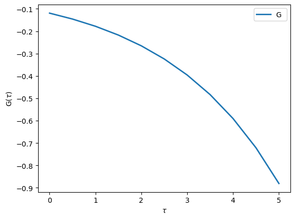
G[tau] = -exp(-tau.value * eps) / (1. + exp(-beta * eps))
print(f"{G[tau]:.3f}")
Green's Function  with mesh Imaginary time mesh with beta = 5, statistics = Fermion, N = 11 and target_shape ():

-0.119
-0.146
-0.178
-0.217
-0.265
-0.324
-0.396
-0.483
-0.590
-0.721
-0.881
In order to plot this Green’s function we can use the matplotlib interface defined in TRIQS. Note that the function to plot Green’s function is oplot and not just plot like in matplotlib.
[5]:
from triqs.plot.mpl_interface import oplot,plt

# Make plots show up directly in the notebook:
%matplotlib inline

# Make all figures slightly bigger
import matplotlib as mpl
mpl.rcParams['figure.dpi']=100

# Additional arguments like 'linewidth' are passed on to matplotlib
oplot(G, '-', name='G', linewidth=2)
Matrix-Valued Green’s functions
In most realistic problems we have to treat more than just a single orbital
For this purpose, TRIQS provides Green’s functions that have a Matrix structure. Let’s see how you can create and use them
[6]:
# A uniform real-frequency mesh on a given interval
from triqs.gfs import MeshReFreq
w_mesh = MeshReFreq(window=(-4,4), n_w=1000)

# Gf with 2x2 Matrix structure holding complex values
G = Gf(mesh=w_mesh, target_shape=[2,2])
for w in w_mesh:
    G[w][0,0] = 1/(w - 0.1 + 1e-5j)
    G[w][1,1] = 1/(w + 0.2 + 1e-5j)

print(G)
Green's Function with mesh Real frequency mesh with w_min = -4, w_max = 4, N = 1000 and target_shape (2, 2):
[7]:
# Accessing a specific mesh point gives us a matrix
from triqs.gfs import Idx # Use Idx to access Gf at specific Index
print(G[Idx(0)])
[[-0.24390244-5.94883998e-07j  0.        +0.00000000e+00j]
 [ 0.        +0.00000000e+00j -0.26315789-6.92520776e-07j]]
[8]:
# By Fixing the orbital indices we obtain a Green's function that is no longer matrix but complex-valued
G[0,0]
[8]:
Green's Function with mesh Real frequency mesh with w_min = -4, w_max = 4, N = 1000 and target_shape ():
Note: ``target_shape=[]`` vs ``target_shape=[1,1]``
These two are not equivalent:
target_shape=[]→ scalar target (target_rank=0), data shape(mesh.size,),G[iw]returns a complex number.target_shape=[1,1]→ 1×1 matrix target (target_rank=2), data shape(mesh.size, 1, 1),G[iw]returns a 1×1 NumPy array.
The practical differences:
Orbital indexing like
G[0,0]is only meaningful for matrix-valued Gf.transpose()andmatrix_transform()requiretarget_rank=2.The two are distinct types on disk, with different data shapes.
Block Green’s functions
In many realistic problems we know a priori that (due to e.g. symmetries or conserved quantum numbers) certain components of the Green’s function will vanish. In other words, the Green’s functions has an additional block structure.
Here the \(\hat{g}^i\) are Green’s functions with non-zero elements \(g^i_{ab}\). In principle they can have different dimensions.
For example, you can imagine a system of 5 \(d\)-orbitals that are split by a crystal field into 3 \(t_{2g}\)-orbitals and 2 \(e_g\)-orbitals. For symmetry reasons, you can have a situation where these orbitals do not talk to each other. In that case, the complete Green’s function would have two blocks, one of size 2x2 corresponding to the \(e_g\) orbitals and one of size 3x3 corresponding for the \(t_{2g}\) orbitals.
Now let’s consider a more concrete example for the case outlined above:
The associated type in TRIQS is called BlockGf. Let us have a first look at it’s documentation:
[9]:
from triqs.gfs import BlockGf
?BlockGf
Python Library Documentation: class BlockGf in module triqs.gfs.block_gf

class BlockGf(builtins.object)
 |  BlockGf(**kwargs)
 |
 |  Block-diagonal Green's function.
 |
 |  A :class:`~triqs.gfs.block_gf.BlockGf` is an **ordered**, named collection of
 |  :class:`~triqs.gfs.gf.Gf` blocks sharing the same mesh and underlying type — for
 |  instance one block per spin or one block per symmetry sector. Block
 |  access uses either the string block name (``g['up']``) or the
 |  positional integer index (``g[0]``). Iteration yields ``(name,
 |  block)`` pairs in construction order.
 |
 |  Three keyword-only constructor patterns are supported (see
 |  Examples):
 |
 |  1. ``BlockGf(name_list=..., block_list=..., make_copies=False, name='G')``
 |     — explicit list of blocks.
 |  2. ``BlockGf(mesh=..., gf_struct=..., target_rank=2, name='G')``
 |     — build matrix-valued blocks from a mesh and block structure.
 |  3. ``BlockGf(name_block_generator=..., make_copies=False, name='G')``
 |     — iterable of ``(name, block)`` pairs.
 |
 |  Parameters
 |  ----------
 |  name_list : list of str, optional
 |      Block names, e.g. ``['up', 'dn']``. Pattern 1 only. Defaults to
 |      ``['0', '1', ...]`` when ``block_list`` is provided.
 |  block_list : list of Gf, optional
 |      One :class:`~triqs.gfs.gf.Gf` per block. Pattern 1 only. All
 |      blocks must have the same Python type.
 |  mesh : Mesh, optional
 |      Common mesh for every block. Pattern 2 only.
 |  gf_struct : list of (str, int), optional
 |      ``(block_name, linear_size)`` pairs. Pattern 2 only.
 |  target_rank : int, optional
 |      Rank of the target space of each block. Pattern 2 only.
 |      Default ``2`` (matrix-valued).
 |  name_block_generator : iterable of (str, Gf), optional
 |      Iterable of ``(name, block)`` pairs. Pattern 3 only.
 |  make_copies : bool, optional
 |      If ``True``, store deep copies of the blocks; otherwise store
 |      the references. Default ``False``.
 |  name : str, optional
 |      Plot label. Default ``'G'``.
 |
 |  Attributes
 |  ----------
 |  name : str
 |      Plot label; also used as a prefix for the individual block
 |      names.
 |  mesh : Mesh
 |      Mesh shared by every block.
 |  beta : float
 |      Inverse temperature of the first block's mesh, when defined.
 |  indices : generator of str
 |      Block names in construction order.
 |  all_indices : generator
 |      Tuples ``(block_name, n1, n2)`` over every entry in every block.
 |  gf_struct : list of (str, int)
 |      Canonical block structure.
 |  n_blocks : int
 |      Number of blocks.
 |  real : BlockGf
 |      Block-wise view of the real part.
 |  imag : BlockGf
 |      Block-wise view of the imaginary part.
 |
 |  Notes
 |  -----
 |  - All blocks must be of the same Python type (e.g. all :class:`~triqs.gfs.gf.Gf`).
 |  - The ``<<`` operator broadcasts lazy initializers / Green's
 |    functions to every block; see :meth:`~triqs.gfs.block_gf.BlockGf.__lshift__`.
 |
 |  Examples
 |  --------
 |  Construct a two-block matrix-valued Matsubara Green's function and
 |  fill every block with a semicircular DOS:
 |
 |  >>> from triqs.gfs import BlockGf, SemiCircular
 |  >>> from triqs.mesh import MeshImFreq
 |  >>> mesh = MeshImFreq(beta=10.0, statistic='Fermion', n_iw=1024)
 |  >>> G = BlockGf(mesh=mesh, gf_struct=[('up', 2), ('dn', 2)])
 |  >>> G << SemiCircular(half_bandwidth=1.0)
 |  >>> for name, g in G:
 |  ...     print(name, g.target_shape)
 |
 |  Methods defined here:
 |
 |  __add__(self, y)
 |      Block-wise addition; returns a new :class:`~triqs.gfs.block_gf.BlockGf`.
 |
 |      Parameters
 |      ----------
 |      y : same as :meth:`~triqs.gfs.block_gf.BlockGf.__iadd__`
 |
 |      Returns
 |      -------
 |      BlockGf
 |
 |  __getitem__(self, key)
 |      Access a block by string name or integer position.
 |
 |      Parameters
 |      ----------
 |      key : str or int
 |          Block name (e.g. ``'up'``) or zero-based block index
 |          (negative integers count from the end).
 |
 |      Returns
 |      -------
 |      Gf
 |          The requested block (a reference, not a copy).
 |
 |      Raises
 |      ------
 |      IndexError
 |          If ``key`` does not name an existing block, or if the
 |          integer is out of range.
 |      TypeError
 |          If ``key`` is neither a ``str`` nor an ``int``.
 |
 |  __iadd__(self, arg)
 |      In-place block-wise addition ``self += arg``.
 |
 |      Parameters
 |      ----------
 |      arg : BlockGf, sequence, or anything accepted by :meth:`~triqs.gfs.gf.Gf.__iadd__`
 |          Same-shape :class:`~triqs.gfs.block_gf.BlockGf` adds block-wise; a sequence
 |          adds element-wise per block; otherwise ``arg`` is
 |          broadcast to every block.
 |
 |      Returns
 |      -------
 |      BlockGf
 |
 |  __imul__(self, arg)
 |      In-place block-wise multiplication ``self *= arg``.
 |
 |      Parameters
 |      ----------
 |      arg : BlockGf or anything accepted by :meth:`~triqs.gfs.gf.Gf.__imul__`
 |
 |      Returns
 |      -------
 |      BlockGf
 |
 |  __init__(self, **kwargs)
 |      Initialize self.  See help(type(self)) for accurate signature.
 |
 |  __isub__(self, arg)
 |      In-place block-wise subtraction ``self -= arg``.
 |
 |      Parameters
 |      ----------
 |      arg : BlockGf, sequence, or anything accepted by :meth:`~triqs.gfs.gf.Gf.__isub__`
 |
 |      Returns
 |      -------
 |      BlockGf
 |
 |  __iter__(self)
 |      Iterate as ``(block_name, block_gf)`` pairs in construction order.
 |
 |      Yields
 |      ------
 |      tuple of (str, Gf)
 |          ``(name, block)`` pairs.
 |
 |  __itruediv__(self, arg)
 |      In-place block-wise division ``self /= arg``.
 |
 |      Parameters
 |      ----------
 |      arg : sequence or scalar
 |          A sequence divides element-wise per block; a scalar is
 |          broadcast.
 |
 |      Returns
 |      -------
 |      BlockGf
 |
 |  __le__(self, other)
 |      Return self<=value.
 |
 |  __len__(self)
 |      Number of blocks.
 |
 |      Returns
 |      -------
 |      int
 |          ``len(self.__GFlist)``.
 |
 |  __lshift__(self, A)
 |      Lazy initialization / copy operator (``G << RHS``).
 |
 |      Parameters
 |      ----------
 |      A : BlockGf, descriptor or Gf-compatible
 |          * If ``A`` is a :class:`~triqs.gfs.block_gf.BlockGf`, copy block-wise.
 |          * If ``A`` is a block descriptor (one yielding per-block
 |            descriptors via ``is_block_descriptor()``), apply each
 |            sub-descriptor to the corresponding block.
 |          * Otherwise broadcast ``A`` to every block: ``g << A`` for
 |            each ``g`` in ``self``.
 |
 |      Returns
 |      -------
 |      BlockGf
 |          ``self`` (so that ``G << RHS`` can be chained).
 |
 |  __mul__(self, y)
 |      Block-wise multiplication; returns a new :class:`~triqs.gfs.block_gf.BlockGf`.
 |
 |      Parameters
 |      ----------
 |      y : BlockGf or anything accepted by :meth:`~triqs.gfs.gf.Gf.__mul__`
 |
 |      Returns
 |      -------
 |      BlockGf
 |
 |  __neg__(self)
 |      Unary minus ``-self``; returns a new :class:`~triqs.gfs.block_gf.BlockGf`.
 |
 |      Returns
 |      -------
 |      BlockGf
 |
 |  __radd__(self, y)
 |      Reflected addition ``y + self``.
 |
 |      Parameters
 |      ----------
 |      y : same as :meth:`~triqs.gfs.block_gf.BlockGf.__add__`
 |
 |      Returns
 |      -------
 |      BlockGf
 |
 |  __reduce__(self)
 |      Helper for pickle.
 |
 |  __reduce_to_dict__(self)
 |
 |  __repr__(self)
 |      Multi-line summary listing every block.
 |
 |      Returns
 |      -------
 |      str
 |          Header line followed by ``repr(g)`` for each block.
 |
 |  __rmul__(self, x)
 |      Reflected multiplication ``x * self``.
 |
 |      Parameters
 |      ----------
 |      x : same as :meth:`~triqs.gfs.block_gf.BlockGf.__mul__`
 |
 |      Returns
 |      -------
 |      BlockGf
 |
 |  __rsub__(self, y)
 |      Reflected subtraction ``y - self``.
 |
 |      Parameters
 |      ----------
 |      y : same as :meth:`~triqs.gfs.block_gf.BlockGf.__sub__`
 |
 |      Returns
 |      -------
 |      BlockGf
 |
 |  __setitem__(self, key, val)
 |      Assign into a block via ``<<``.
 |
 |      ``G[key] = val`` is equivalent to ``G[key] << val``.
 |      ``G[:] = val`` is equivalent to ``G << val`` (broadcast to every
 |      block).
 |
 |      Parameters
 |      ----------
 |      key : str, int or slice
 |          Block selector. ``slice(None, None, None)`` broadcasts.
 |      val : Gf, BlockGf, descriptor or scalar
 |          Value to assign.
 |
 |  __str__(self)
 |      Alias for :meth:`~triqs.gfs.block_gf.BlockGf.__repr__`.
 |
 |      Returns
 |      -------
 |      str
 |
 |  __sub__(self, y)
 |      Block-wise subtraction; returns a new :class:`~triqs.gfs.block_gf.BlockGf`.
 |
 |      Parameters
 |      ----------
 |      y : same as :meth:`~triqs.gfs.block_gf.BlockGf.__isub__`
 |
 |      Returns
 |      -------
 |      BlockGf
 |
 |  __truediv__(self, y)
 |      Block-wise division; returns a new :class:`~triqs.gfs.block_gf.BlockGf`.
 |
 |      Parameters
 |      ----------
 |      y : same as :meth:`~triqs.gfs.block_gf.BlockGf.__itruediv__`
 |
 |      Returns
 |      -------
 |      BlockGf
 |
 |  conjugate(self)
 |      Complex-conjugate every block.
 |
 |      Returns
 |      -------
 |      BlockGf
 |          New container holding the complex conjugate of every block
 |          of ``self``.
 |
 |  copy(self, *args)
 |      Return an independent deep copy of ``self`` (every block is copied).
 |
 |      Parameters
 |      ----------
 |      *args
 |          Forwarded to the per-block ``copy()`` method.
 |
 |      Returns
 |      -------
 |      BlockGf
 |          Independent copy with freshly allocated blocks.
 |
 |  copy_from(self, G2)
 |      Copy the data of ``G2`` into ``self`` block by block.
 |
 |      Parameters
 |      ----------
 |      G2 : BlockGf
 |          Source container. Must have the same number of blocks in
 |          the same order and identical per-block ``target_shape``.
 |
 |      Raises
 |      ------
 |      RuntimeError
 |          If any pair of blocks has incompatible target shape.
 |
 |  copy_selected_blocks(self, selected_blocks)
 |      Return a new :class:`~triqs.gfs.block_gf.BlockGf` containing **deep copies** of the named blocks.
 |
 |      Parameters
 |      ----------
 |      selected_blocks : sequence of str
 |          Block names to copy.
 |
 |      Returns
 |      -------
 |      BlockGf
 |          New container with independent copies of the requested
 |          blocks.
 |
 |  density(self, *args, **kwargs)
 |      Compute per-block single-particle density matrices.
 |
 |      Equivalent to :math:`\langle c^\dagger_i c_j \rangle` evaluated
 |      per block from the diagonal-frequency / equal-time limit of the
 |      block Green's function.
 |
 |      Parameters
 |      ----------
 |      *args, **kwargs
 |          Forwarded to :meth:`~triqs.gfs.gf.Gf.density` for each block.
 |
 |      Returns
 |      -------
 |      dict of {str : numpy.ndarray}
 |          Mapping ``block_name -> density_matrix``.
 |
 |  inverse(self)
 |      Compute the inverse of every block.
 |
 |      Returns
 |      -------
 |      BlockGf
 |          New container holding the matrix/scalar inverse of every
 |          block of ``self``.
 |
 |  invert(self)
 |      Invert each block in place.
 |
 |  load(self, filename, no_exception=False)
 |      Load each block from a text file ``filename_<blockname>``.
 |
 |      Parameters
 |      ----------
 |      filename : str
 |          Common prefix.
 |      no_exception : bool, optional
 |          If ``True``, silently skip blocks whose file cannot be read.
 |          Default ``False``.
 |
 |  save(self, filename, accumulate=False)
 |      Save each block to a text file ``filename_<blockname>``.
 |
 |      Parameters
 |      ----------
 |      filename : str
 |          Common prefix; each block is written to
 |          ``"{filename}_{block_name}"``.
 |      accumulate : bool, optional
 |          Forwarded to the per-block ``save`` method. Default
 |          ``False``.
 |
 |  total_density(self, *args, **kwargs)
 |      Compute the total density summed over all blocks.
 |
 |      Parameters
 |      ----------
 |      *args, **kwargs
 |          Forwarded to :meth:`~triqs.gfs.gf.Gf.total_density` for each block.
 |
 |      Returns
 |      -------
 |      float or complex
 |          Sum of ``g.total_density(...)`` over every block.
 |
 |  transpose(self)
 |      Transpose every block in target space.
 |
 |      Returns
 |      -------
 |      BlockGf
 |          New container holding the target-space transpose of every
 |          block of ``self``.
 |
 |  view_selected_blocks(self, selected_blocks)
 |      Return a new :class:`~triqs.gfs.block_gf.BlockGf` containing **views** of the named blocks.
 |
 |      Parameters
 |      ----------
 |      selected_blocks : sequence of str
 |          Block names to expose. Must all exist in ``self``.
 |
 |      Returns
 |      -------
 |      BlockGf
 |          New container holding view-references to the requested
 |          blocks, in their original order.
 |
 |  zero(self)
 |      Set every block's data to zero, in place.
 |
 |  ----------------------------------------------------------------------
 |  Class methods defined here:
 |
 |  __factory_from_dict__(name, d)
 |
 |  ----------------------------------------------------------------------
 |  Readonly properties defined here:
 |
 |  all_indices
 |      Iterate over flat indices ``(block_name, n1, n2)`` for every matrix-valued block.
 |
 |      Yields
 |      ------
 |      tuple of (str, int, int)
 |          ``(block_name, n1, n2)`` triple.
 |
 |  beta
 |      Inverse temperature :math:`\beta`.
 |
 |      Returns
 |      -------
 |      float
 |          :math:`\beta`.
 |
 |  gf_struct
 |      Canonical block structure.
 |
 |      Returns
 |      -------
 |      list of (str, int)
 |          ``(block_name, linear_size)`` for every block.
 |
 |  imag
 |      Block-wise view of the imaginary part.
 |
 |      Returns
 |      -------
 |      BlockGf
 |          New container holding ``g.imag`` for each block; the
 |          ``name`` is prefixed with ``'Im '`` when ``self.name`` is
 |          non-empty.
 |
 |  indices
 |      Block names in construction order.
 |
 |      Yields
 |      ------
 |      str
 |          Block name.
 |
 |  mesh
 |      Mesh shared by every block.
 |
 |      Returns
 |      -------
 |      Mesh
 |          Mesh shared by every block (read from the first block).
 |
 |      Notes
 |      -----
 |      Deprecated; access ``g.mesh`` on individual blocks instead.
 |
 |  n_blocks
 |      Number of blocks.
 |
 |      Returns
 |      -------
 |      int
 |          ``len(self.__GFlist)``.
 |
 |  real
 |      Block-wise view of the real part.
 |
 |      Returns
 |      -------
 |      BlockGf
 |          New container holding ``g.real`` for each block; the
 |          ``name`` is prefixed with ``'Re '`` when ``self.name`` is
 |          non-empty.
 |
 |  ----------------------------------------------------------------------
 |  Data descriptors defined here:
 |
 |  __dict__
 |      dictionary for instance variables
 |
 |  __weakref__
 |      list of weak references to the object
 |
 |  ----------------------------------------------------------------------
 |  Data and other attributes defined here:
 |
 |  __array_priority__ = 10000
We will in the following consider the first two options for the construction listed in the documentation.
The first way is to simply define the two Green’s function blocks separately, and to then pass these blocks, together with their names:
[10]:
# Construct individual blocks
g_eg  = Gf(mesh=w_mesh, target_shape=[2,2])
g_t2g = Gf(mesh=w_mesh, target_shape=[3,3])

# Combine blocks into a BlockGf
G = BlockGf(name_list=['eg', 't2g'], block_list=[g_eg, g_t2g])
print(G)
Green Function G composed of 2 blocks:
 Green's Function G_eg with mesh Real frequency mesh with w_min = -4, w_max = 4, N = 1000 and target_shape (2, 2):

 Green's Function G_t2g with mesh Real frequency mesh with w_min = -4, w_max = 4, N = 1000 and target_shape (3, 3):
We can then access individual blocks simply by using their name
[11]:
G['eg']
[11]:
Green's Function G_eg with mesh Real frequency mesh with w_min = -4, w_max = 4, N = 1000 and target_shape (2, 2):
For cases where all blocks have a square-matrix target_shape we can alternatively pass a list of pairs of block-names and linear matrix sizes.
[12]:
# List of Block-names and their linear matrix size
gf_struct = [('eg',2), ('t2g',3)]

G = BlockGf(mesh=w_mesh, gf_struct=gf_struct)
print(G)
Green Function G composed of 2 blocks:
 Green's Function G_eg with mesh Real frequency mesh with w_min = -4, w_max = 4, N = 1000 and target_shape (2, 2):

 Green's Function G_t2g with mesh Real frequency mesh with w_min = -4, w_max = 4, N = 1000 and target_shape (3, 3):
Now let’s initialize the Green’s function values. Instead of writing a loop over the mesh, we here make use of the the operator <<, which can fill the Green’s function with simple expressions containing the Omega descriptor. Here Omega takes all values of the mesh.
Note: The loop initialization is recommended for more complicated expressions involving e.g. calls to math functions
[13]:
from triqs.gfs import Omega

V1 = 0.1
V2 = 0.2
eps_t2g = -2.0
ieta = 1e-13j

# The e_g part
G['eg'][0,0] << Omega + ieta
G['eg'][0,1] << V1
G['eg'][1,0] << V1
G['eg'][1,1] << Omega + ieta

# Perform an in-place Matrix inversion
G['eg'].invert()

# The t_2g part
G['t2g'][0,0] << Omega - eps_t2g + ieta
G['t2g'][1,1] << Omega - eps_t2g + ieta
G['t2g'][2,2] << Omega - eps_t2g + ieta
G['t2g'][0,2] << V2
G['t2g'][2,0] << V2
G['t2g'].invert()
When using the Green’s function object, it is often convenient to iterate over all the blocks of a BlockGf. We can do this with the following construct
[14]:
# Loop over the blocks
for name, g in G:
    print("This is the block called", name)
    print("The associated Green's function is", g)
This is the block called eg
The associated Green's function is Green's Function G_eg with mesh Real frequency mesh with w_min = -4, w_max = 4, N = 1000 and target_shape (2, 2):

This is the block called t2g
The associated Green's function is Green's Function G_t2g with mesh Real frequency mesh with w_min = -4, w_max = 4, N = 1000 and target_shape (3, 3):
Additional Initialization Descriptors
In the following we will introduce a few additional means of initializing Green’s functions using <<.
Flat density of states
Consider the problem of a single atomic level embedded in a flat conduction bath \(\Gamma\) of electrons.
In the equation above \(\epsilon_d\) is the energy of the level and \(\Gamma\) is the Green’s function of a flat conduction bath as obtained via the Hilbert transform
Here \(D\) denotes the half-bandwidth and \(\rho(\omega) = \theta(D-|\omega|)/(2D)\) is the density of states.
Let’s see how to define and then plot this Green’s function by using inverse and the Flat descriptor.
[15]:
eps_d = 1.0 # Energy
V = 0.2   # Bath Hybridization
D = 1.5   # Half bandwidth

G = Gf(mesh=w_mesh, target_shape=[])

from triqs.gfs import Omega, Flat, inverse
G << inverse(Omega - eps_d - V**2 * Flat(D) + ieta)
[15]:
Green's Function with mesh Real frequency mesh with w_min = -4, w_max = 4, N = 1000 and target_shape ():
Note the predefined function Flat for a flat conduction bath \(\Gamma(\omega)\). Let’s plot the atomic Green’s function. Note that default, both the real and imaginary parts are plotted.
[16]:
oplot(G, '-', linewidth=2, name="G")
We can plot the spectral function, which is defined as
[17]:
from math import pi
oplot(-G.imag/pi, linewidth=2, name=r"$\rho$")
As expected the spectral function is peaked at \(\epsilon_d\) and shows a jump in spectral weight at \(D\).
Semi-circular density of states
Another predefined Green’s function is the one corresponding to a semi-circular spectral function. This one will be useful in the DMFT Tutorials later on.
[18]:
D = 1.0 # Half bandwidth

G = Gf(mesh=w_mesh, target_shape=[])

from triqs.gfs import SemiCircular
G << SemiCircular(D)

oplot(-G.imag/pi, name=r"$\rho$")
Imaginary-frequency Green’s functions
These are Green’s function defined on the Matsubara axis. The fermionic Matsubara frequencies are defined by
where \(\beta = 1/T\) is the inverse temperature. These Green’s functions are important because most Monte Carlo algorithms yield results on the Matsubara axis. Let’s see how they are defined:
[19]:
# Define the imaginary-frequency mesh
from triqs.gfs import MeshImFreq
iw_mesh = MeshImFreq(beta=5, statistic='Fermion', n_iw=1000)

# Create Green's function and fill it using the iOmega_n descriptor
G = Gf(mesh=iw_mesh, target_shape=[])
from triqs.gfs import iOmega_n
G << inverse(iOmega_n - 0.2)

# Plot the Green's function
oplot(G, '-o', name='G')
plt.xlim(0,10)
[19]:
(0.0, 10.0)
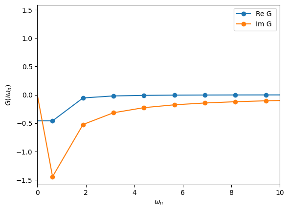
Arithmetic Operations
Green’s functions can be added, multiplied by numbers, etc. The way this is done is quite natural.
[20]:
oplot(G, "-o", name='G')
oplot(G+G, "-o", name='G+G')
oplot(3*G+2, "-o", name='3*G+2')
plt.xlim(0,10)
[20]:
(0.0, 10.0)
Obtaining the density
You can obtain the density for Green’s functions with a MeshReFreq and MeshImFreq using the density method
[21]:
G = Gf(mesh=iw_mesh, target_shape=[])
G << inverse(iOmega_n - 0.2)
print("Density =", G.density())
Density = (0.2689414213802603-2.867555569693999e-15j)
Do not worry about the imaginary component as the machine precision is on the order of \(10^{-15}\).
Fourier transforms
TRIQS allows you to easily Fourier transform Green’s functions from imaginary-time to imaginary-frequency.
[22]:
# A Green's function in frequency set to semi-circular
Giw = Gf(mesh=iw_mesh, target_shape=[])
Giw << SemiCircular(1.0)

# A Green's function in time set by inverse Fourier transform
from triqs.gfs import make_gf_from_fourier
Gtau = make_gf_from_fourier(Giw)
oplot(Gtau, name='G')
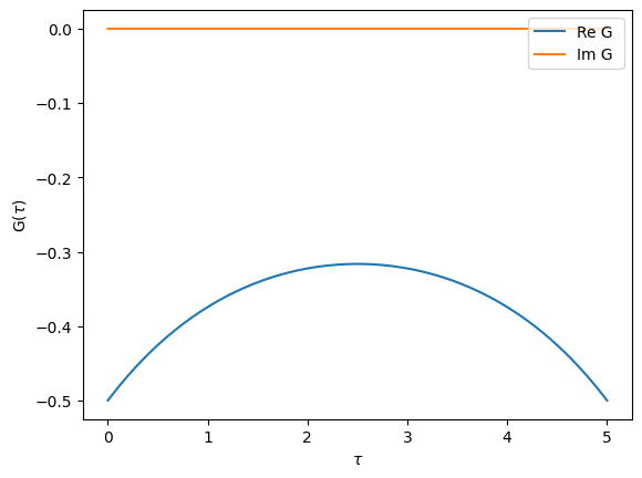
We can also go the other way. Let’s check that it gives back the original result.
[23]:
Giw_2 = make_gf_from_fourier(Gtau)
oplot(Giw, 'o')
oplot(Giw_2, 'x')
plt.xlim(0,5)
[23]:
(0.0, 5.0)
In the example above make_gf_from_fourier will construct a new Green’s function object. This uses the statistic information of MeshImTime to decide whether to use bosonic or fermionic Matsubara frequencies. If we want to instead use an existing Green’s function we can use the Fourier descriptor
[24]:
from triqs.gfs import Fourier
Gtau << Fourier(Giw)
[24]:
Green's Function with mesh Imaginary time mesh with beta = 5, statistics = Fermion, N = 6001 and target_shape ():
Compact meshes for imaginary time / frequency: DLR Green’s function
When representing Green’s functions at low temperatures the regular meshes MeshImFreq and MeshImTime may easily require several thousand of points to store the relevant information. This is often problematic when storing or initializing lattice Green’s functions with a momentum and orbital dependence.
For this purpose TRIQS provides mesh types on the Matsubara / imaginary time axis that are much more compact, based on the Discrete Lehman Representation (DLR), for a detailed introduction see Kaye et al., PRB105, 2022.
The DLR of an imaginary time Green’s function is given by an expansion of the form
where \(K(\tau,\omega) = -\frac{e^{-\tau \omega}}{1+e^{-\beta \omega}}\) is the analytic continuation kernel appearing in the spectral Lehmann representation
relating \(G\) to its spectral density \(\rho\).
The DLR frequencies \(\omega_l\) are obtained by a numerical scheme that is independent of the specific Green’s function \(G\). They depend only on the desired accuracy \(\epsilon\) of the DLR expansion, and a dimensionless cutoff parameter \(\Lambda = \beta \omega_{max}\) characterized by the assumption that \(\rho(\omega) = 0\) outside of the interval \([-\omega_{max}, \omega_{max}]\). The DLR basis is one of the most compact representations of Matsubara Green’s functions and the basis size scales only logarithmically with \(\beta\).
To get started we first create a Matsubara Green’s function with a SemiCircular density of states function at a low temperature of \(\beta=100\). For the imaginary part of G to decay to zero we have to use as many as ~1500 Matsubara frequencies.
[25]:
iw_mesh = MeshImFreq(beta=100, statistic='Fermion', n_iw=1500)
Giw = Gf(mesh=iw_mesh, target_shape=[])
Giw << SemiCircular(1.0)
[25]:
Green's Function with mesh Imaginary frequency mesh with beta = 100, statistics = Fermion, N_iw = 1500, positive_only = false and target_shape ():
We now construct a DLR Matsubara Green’s function. Similar to the MeshImFreq we have to provide \(\beta\) and the particle statistics. Additionally we set the maximal spectral width of the Green’s function w_max (half spectral width), plus the precision we want to achieve with the DLR basis:
[26]:
# import DLR mesh
from triqs.mesh import MeshDLRImFreq

dlr_iw_mesh = MeshDLRImFreq(beta=100, statistic='Fermion', w_max=1.2, eps=1e-12)
# the Gf is constructed then the same way
Giw_dlr = Gf(mesh= dlr_iw_mesh, target_shape=[])

print(dlr_iw_mesh)
DLR imaginary frequency mesh of size 36 with beta = 100, statistics = Fermion, w_max = 1.2, eps = 1e-12, symmetrized = true
By printing the mesh we see that its size is 36 which is substantially smaller than 1500. We can initialize the DLR Matsubara Green’s function using the same syntax as before
[27]:
Giw_dlr << SemiCircular(1.0);
Let us now plot both Green’s functions:
[28]:
fig, ax = plt.subplots(1,figsize=(12,5))
oplot(Giw, "-", name='G')
oplot(Giw_dlr, name='G DLR')
plt.xlim(-0.1,94)
plt.ylim(-2,0.1)
plt.legend(loc='lower right');
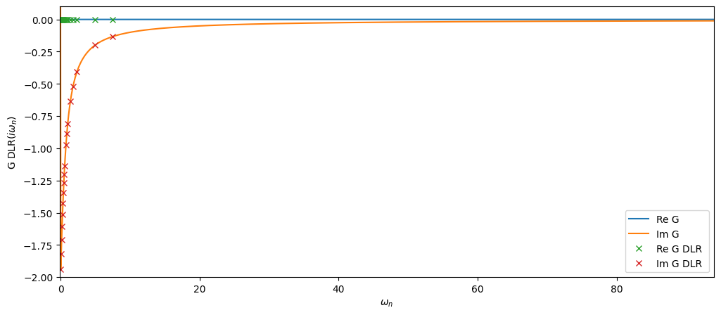
The DLR mesh Matsubara nodes are quite sparse but as we will see below the data is sufficient to reconstruct the full Matsubara mesh up to the precision specified.
Next we create the DLR coefficient Green’s function associated with Giw_dlr. This form is central as it can be easily converted into a Gf with any of the mesh types MeshImTime, MeshImFreq, MeshDLRImTime and MeshDLRImFreq.
We obtain the Green’s function on the full Matsubara mesh using the function make_gf_imfreq to then compare it against the original Giw.
[29]:
# import helper functions
from triqs.gfs import make_gf_dlr, make_gf_dlr_imtime, make_gf_imfreq, make_gf_imtime

# create DLR coefficient Green's function
G_dlr = make_gf_dlr(Giw_dlr)

# Get back Green's function on the full Matsubara mesh, no Fourier transform needed
Giw_from_dlr = make_gf_imfreq(G_dlr, n_iw=1500)

# plot the difference between the original
fig, ax = plt.subplots(1,figsize=(7,5))

mesh = [iw.imag for iw in Giw.mesh.values()]
ax.plot(mesh, abs((Giw_from_dlr-Giw).data))
ax.semilogy()
ax.set_xlim(0,94)
ax.set_xlabel(r'$i\omega_n$')
ax.set_ylabel(r'$|G_{ref}-G_{DLR}|$');
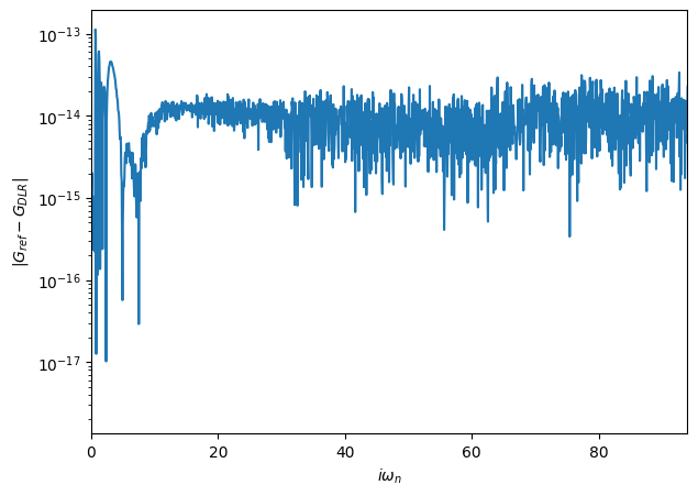
The given accuracy eps=1e-12 is reached over the full Matsubara mesh!
The coefficient DLR mesh Gf can be evaluated on any given tau point by passing the Gf a float:
[30]:
G_dlr(1.2)
[30]:
(-0.31556737050746025-1.840192666076156e-17j)
or on the Matsubara axis by passing a Matsubara mesh point:
[31]:
G_dlr(iw_mesh(0))
[31]:
(-5.411651148360362e-17-1.9381548639656863j)
Finally we can also construct an imaginary time Green’s functions, using make_gf_dlr_imtime on the compact mesh, and using make_gf_imtime on arbitrarily dense \(\tau\) meshes by passing the parameter n_tau:
[32]:
Gtau_dlr = make_gf_dlr_imtime(G_dlr)
Gtau = make_gf_imtime(G_dlr, n_tau=5001)

oplot(Gtau_dlr.real, name='G DLR')
oplot(Gtau.real, name='G')
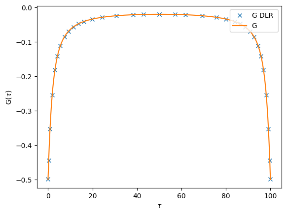
Pade analytical continuation
The Fourier transforms allow to go from time to frequency. A much more delicate thing is to do the so-called “analytical continuation”. This means to start from a Matsubara-frequency Green’s function and obtain the corresponding real-frequency Green’s function. This can formally be done, but turns out to be a mathematically ill-conditioned problem. Even small amounts of noise in the Matsubara-frequency data will make the continuation to the real axis very unstable.
One of the ways to do perform analytical continuation is to use Pade approximants. TRIQS can do that for you in the following way:
Note: Pade is currently implemented only for Green’s functions with a Matrix structure
[33]:
# The Matsubara Green's function to be continued
iw_mesh = MeshImFreq(beta=50, statistic='Fermion', n_iw=1000)
Giw = Gf(mesh=iw_mesh, target_shape=[])
Giw << SemiCircular(1.0)

# Construct real-frequency Green's function and initialize it using Pade approximants
Gw = Gf(mesh=w_mesh, target_shape=[])
Gw.set_from_pade(Giw)

oplot(-Gw.imag/pi, linewidth=2)
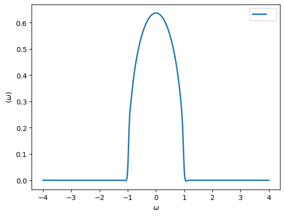
The coarse Matsubara discretization at high temperatures will worsen the Pade result, which is why we chose a much lower temperature value for this example.
You can see that the Pade continuation did a pretty good job. We will see later that noise will completely change this picture!
Exercises
Exercise 1
Define the following real-frequency Green’s function, where \(\Gamma\) is the Green’s function of a flat bath (width = 1), \(\epsilon_d = 0.3\) and \(V=0.2\):
Plot the spectral function for both diagonal components of this Green’s function. What do they represent physically?
[34]:
# Parameters
eps_d, V = 0.3, 0.2

# Construct and Initialize Gf
w_mesh = MeshReFreq(window=(-2,2), n_w=1000)
G = Gf(mesh=w_mesh, target_shape=[2,2])
G[0,0] << Omega - eps_d + ieta
G[0,1] << V
G[1,0] << V
G[1,1] << inverse(Flat(1.0))
G.invert()

# Plot
oplot(-G[0,0].imag/pi, '-', lw=2, name = "Impurity")
oplot(-G[1,1].imag/pi, '-', lw=2, name = "Bath")
Exercise 2
Plot the density \(n(\epsilon)\) as a function of \(\epsilon\) for a Green’s function \(G = 1/(i\omega_n - \epsilon)\). What is the curve that you obtained? How does it change with temperature?
[35]:
# Consider various temperatures
for beta in [3, 10, 100]:

    # Construct Gf
    iw_mesh = MeshImFreq(beta=beta, statistic='Fermion', n_iw=1000)
    G = Gf(mesh=iw_mesh, target_shape=[])

    # Initialize and plot for different epsilon
    import numpy
    eps_r = numpy.arange(-1,1,0.05)
    n_r = []
    for eps in eps_r:
        G << inverse(iOmega_n - eps)
        n_r.append(G.density().real)
    plt.plot(eps_r, n_r, lw=2, label=rf'$\beta = {beta}')

plt.xlabel(r'$\epsilon$')
plt.ylabel(r'$n(\epsilon)$')
plt.legend()
[35]:
<matplotlib.legend.Legend at 0x146145f05550>
Exercise 3
Define a block Green’s function with an up and a down block. Each block is just a simple 1x1 imaginary-frequency Green’s function. Iterate over the blocks to initialize the two blocks to \(1/i \omega_n\). What happens if you change \(\beta\)?
[36]:
# Consider various temperatures
for beta in [5, 7, 10]:
    iw_mesh = MeshImFreq(beta=beta, statistic='Fermion', n_iw=1000)
    G = BlockGf(mesh=iw_mesh, gf_struct=[('up',1),('down',1)])

    # Loop over the blocks to initialize
    for name, g in G:
        g << inverse(iOmega_n)

    # Plot one entry
    oplot(G["up"][0,0].imag, '-o', name=rf"Im G[$\beta$={beta}]")

plt.xlim(0,5)
plt.ylim(-3.5,0.1)
plt.ylabel(r"Im G[$\beta$]")
[36]:
Text(0, 0.5, 'Im G[$\\beta$]')
Exercise 4
Consider a Hubbard atom with \(U=2\) at temperature \(T = 1/\beta = 1/10\). The non-interacting and interacting Green’s functions for this problem are:
Here the chemical potential \(\mu\) is chosen such that the interacting system is half filled.
Using Dyson’s equation, verify that the corresponding self-energy is indeed
Note: At half-filling the chemical potential :math:`mu = U/2` and the static part of the self-energy exactly cancel.
[37]:
# Parameters
U = 2.0

# Green's function containers
iw_mesh = MeshImFreq(beta=10, statistic='Fermion', n_iw=1000)
G_0 = Gf(mesh=iw_mesh, target_shape=[])
G = G_0.copy()
Sigma = G_0.copy()
Sigma_check = G_0.copy()

# Green's functions of the Hubbard atom
G_0 << inverse(iOmega_n + U/2)
G << 0.5*inverse(iOmega_n + U/2) + 0.5*inverse(iOmega_n - U/2)

# Dyson's equation to find the self-energy
Sigma << inverse(G_0) - inverse(G)

# Known solution
Sigma_check << U/2 + U**2 * inverse(4*iOmega_n)

oplot(Sigma_check, '-o', name=r'$\Sigma$_check')
oplot(Sigma, '-x', name=r'$\Sigma$')
plt.xlim(0,10)
[37]:
(0.0, 10.0)
Exercise 5
Compute the following second-order self-energy with \(U=2\) and \(\beta=50\)
using an non-interacting \(G_0\) given by a semi-circular of half-bandwidth 1. Use Dyson’s equation to compute \(G(i\omega_n)\).
Note that here we have neglected the static part of the self-energy, as at half-filling we assume the chemical potential to exactly cancel it.
Hint: The SemiCircular initializer only works for frequency Green’s functions.
Hint: The “power operator” is not defined for Green’s functions. Use multiplication.
[38]:
# Parameters
U = 2.0

# Define and initialize G0 in freq
iw_mesh = MeshImFreq(beta=50, statistic='Fermion', n_iw=1000)
G0_iw = Gf(mesh=iw_mesh, target_shape=[1,1])
G0_iw << SemiCircular(1.0)

# Compute second-order self-energy
G0_tau = make_gf_from_fourier(G0_iw)
Sigma_tau = U**2 * G0_tau * G0_tau * G0_tau
Sigma_iw = make_gf_from_fourier(Sigma_tau)

# Dyson's equation
G_iw = G0_iw.copy()
G_iw << inverse(inverse(G0_iw) - Sigma_iw)

oplot(G_iw, '-o', name='G')
plt.xlim(0,4)
[38]:
(0.0, 4.0)
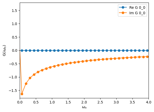
Exercise 6
Use Pade approximants to obtain a real-frequency version of the Green’s function computed in the Exercise 5. What is the effect of interactions at second-order perturbation theory? How is it changing with different values of \(U\)?
[39]:
# Create Green's functions
w_mesh = MeshReFreq(window=(-4,4), n_w=1000)
G_w = Gf(mesh=w_mesh, target_shape=[1,1])
G0_w = G_w.copy()

# Initialize from Pade
G_w.set_from_pade(G_iw)
oplot(-G_w[0,0].imag/pi, lw=2, name="Second-order")

# Initialize non-interacting Green's function
G0_w << SemiCircular(1.0)
oplot(-G0_w[0,0].imag/pi, name="Non-interacting")

plt.ylabel(r"$\rho(\omega)$")
[39]:
Text(0, 0.5, '$\\rho(\\omega)$')
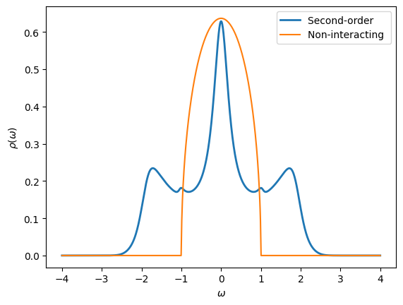
The interaction leads to a shift of spectral weight towards a low- and a high-energy feature, often referred to as the lower and upper Hubbard band. These features move outwards with increasing interaction strength.