Manipulating fermionic operators

Before we see how to use a CTQMC impurity solver, let’s learn about operators. Indeed, one of the inputs of the CTQMC solver is a Hamiltonian in operator form.

Fundamental operators

After importing the operator module, the keyword c_dag and c allow to define a new fermionic operator. c_dag and c are followed by two indices. Inspired by the block structure of Green’s functions, the first index is a block index, while the second is the index within the block. Here’s an example of operators as they would be defined if we had two blocks up and down of size 1:

from triqs.operators import c, c_dag, n, Operator # n and Operator will be needed later
print(c_dag('up',0))
print(c('up',0))
print(c_dag('down',0))
print(c('down',0))

1*c_dag('up',0)
1*c('up',0)
1*c_dag('down',0)
1*c('down',0)

Number operator

The keyword n is defined as \(C^\dagger C\)

print(n('up',0))

1*c_dag('up',0)*c('up',0)

Operations with operators

Operators can be manipulated and anti-commutation relations will be used to simplify expressions

# Should give 0
print(n('up',0) - c_dag('up',0)*c('up',0))

0

# Some calculation
print(n('up',0) - 2 * c_dag('up',0)*c('up',0))

-1*c_dag('up',0)*c('up',0)

# Define the parameters
U = 4
mu = 3

# H is an empty operator
H = Operator()

# Add elements to define a Hamiltonian
H += U * n('up',0) * n('down',0)
H -= mu * (n('up',0) + n('down',0))
print(H)

-3*c_dag('down',0)*c('down',0) + -3*c_dag('up',0)*c('up',0) + 4*c_dag('down',0)*c_dag('up',0)*c('up',0)*c('down',0)

Exact Diagonalization

For small system-sizes we can use AtomDiag provided by TRIQS to perform exact diagonalization on the Hamiltonian

from triqs.atom_diag import AtomDiag
?AtomDiag

Python Library Documentation: function AtomDiag in module triqs.atom_diag

AtomDiag(*args, **kwargs)
    Construct an exact diagonalization solver, dispatched on the Hamiltonian type.

    Returns :class:`AtomDiagReal` when the Hamiltonian (and any further operator
    arguments) is purely real, and :class:`AtomDiagComplex` otherwise. The
    arguments are forwarded unchanged to the chosen class constructor; see
    :class:`AtomDiagReal` for the full list of supported overloads.

    Parameters
    ----------
    h : Operator
        Many-body Hamiltonian to be diagonalized.
    *args, **kwargs
        Additional positional and keyword arguments forwarded to the
        :class:`AtomDiagReal` / :class:`AtomDiagComplex` constructor (e.g.
        ``fops``, ``hyb``, ``n_min``/``n_max`` or ``qn_vector``).

    Returns
    -------
    AtomDiagReal or AtomDiagComplex
        Solved diagonalization problem.

# List of operator flavors
fops = [('up',0), ('down',0)]

# Construct AtomDiag object, Performs diagonalization
AD = AtomDiag(h=H, fops=fops)

print(AD.gs_energy)

-3.0

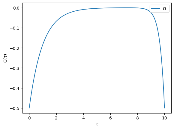
We can then use the AtomDiag object to obtain for example the atomic Green’s functions

from triqs.atom_diag import atomic_g_tau
Gtau = atomic_g_tau(atom=AD, beta=10, gf_struct=[('up',1),('down',1)], n_tau=1001)

from triqs.plot.mpl_interface import oplot
%matplotlib inline
oplot(Gtau["up"][0,0].real, name='G')