Introduction to multivariable Green’s functions
This notebook demonstrates how to create and manipulate multivariable Green’s functions. As an example, we consider the Green’s function on a square lattice with nearest-neighbour hopping \(t\),
\begin{equation} G(\mathbf{k},i\omega_n)=\frac{1}{i\omega_n + \mu - \epsilon(\mathbf{k})} \end{equation}
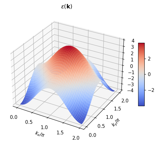
with dispersion \(\epsilon(\mathbf{k})=-2t(\cos{k_x}+\cos{k_y})\). Here \(\mathbf{k}\) is a vector in the Brillouin zone (in units where the lattice spacing is unity \(a=1\)), \(\mu\) is the chemical potential and \(i\omega_n\) is a Matsubara frequency.
Imports and parameters
Below we import modules that will be useful in the following. We also set the parameters of the problem.
[1]:
# Relevant Imports
from triqs.lattice import BravaisLattice, BrillouinZone
from triqs.gfs import Gf, MeshProduct, MeshBrZone, MeshImFreq
import numpy as np
from math import cos, pi
[2]:
# Physical parameters
beta = 2     # Inverse temperature
t = 1.0      # Hopping (unit of energy)
mu = 0       # Chemical potential
Constructing and Initializing a Lattice Green’s function
We first define a simple Bravais lattice (BravaisLattice) in 2 dimensions with basis vectors \(\hat{e}_x = (1, 0, 0)\) and \({\hat e}_y=(0, 1, 0)\). Given this bravais lattice we construct the reciprocal (momentum) space Brillouin zone (BrillouinZone), on which we can then construct a momentum mesh (MeshBrZone).
[3]:
BL = BravaisLattice([(1,0,0), (0,1,0)]) # Two unit vectors in R3
BZ = BrillouinZone(BL)

# n_k denotes the number of k-points for each dimension
n_k = 128
k_mesh = MeshBrZone(bz=BZ, n_k=n_k)
The Lattice Green’s function is defined on a mesh that is the cartesian product of this momentum mesh and a Matsubara mesh.
To construct this mesh we use the MeshProduct provided by TRIQS:
[4]:
iw_mesh = MeshImFreq(beta=beta, statistic='Fermion', n_iw=128)
k_iw_mesh = MeshProduct(k_mesh, iw_mesh)

# Recall that for an empty target_shape G0 has values that are scalars instead of matrices.
G = Gf(mesh=k_iw_mesh, target_shape=[])
To fill the Green’s function we construct a function for the dispersion \(\epsilon(\mathbf{k})\) and set each element of \(G\) by looping over the momentum and frequency meshes.
[5]:
#%%timeit
def eps(k):
    return -2*t * (cos(k[0]) + cos(k[1]))

# Loop initialization. Slow..
for k, iw in G.mesh:
    G[k, iw] = 1/(iw + mu - eps(k))
NumPy Broadcasting
Instead of writing a loop we can use the broadcasting features of the NumPy package to assign directly into the data-array of the Green’s function object. This approach is a lot faster than writing a loop
[6]:
iw_arr = np.array(list(iw_mesh.values()))
k_arr  = np.array(list(k_mesh.values()))
np_eps = np.vectorize(eps, signature='(d)->()')
[7]:
#%%timeit
# Vectorized function evaluation
eps_arr = np_eps(k_arr)

# Numpy Broadcasting
G.data[:] = 1.0 / (iw_arr[None,::] + mu - eps_arr[::,None])
We provide through the TRIQS/tprf application more efficient parallelized routines for initializing lattice Green functions. Those will be introduced in the Two Particle Reponse Notebooks.
Evaluate the Green’s function
The Green’s function object \(G(k,i\omega_n)\) can be evaluated like an ordinary Python function at a given reciprocal vector and Matsubara frequency:
The reciprocal vector \(k\) is a tuple/list/numpy.array of double
The Matsubara frequency is an integer \(n\), the \(n\) in \(i\omega_n\)
The result will be a linear interpolation on the Brillouin zone with the points on the grid of \(G\) around \(k\).
Therefore, one can use \(g_0\) as any python function of \(k\) and \(i\omega_n\), and forget its precise representation in memory (what is the grid, etc…). We will use that in the plot functions below.
Example: Let’s evaluate the above Green’s function at \(\mathbf{k} = (\pi,\pi,0)\) and \(i\omega_2\). As \(\epsilon((\pi,\pi,0)) = 4t = 4\) and \(i\omega_2 = i\frac{(2*2 + 1)\pi}{\beta}\), we check:
[8]:
G_eval  = G((pi,pi,0), 2)
G_exact = 1.0/(1j * (2*2+1)*pi/beta - 4)
print(G_eval - G_exact) # Check
0j
Partial evaluation
Given a function \(G(k,i\omega_n)\) you can obtain the function \(i\omega_n \rightarrow G(k_0, i\omega_n)\) for a fixed \(k_0\):
[9]:
k0 = (0.02,0.01,0)      # a k-point as a tuple of 3 floats
Giw = G(k0, all)        # We use the "built-in" function all here as equivalent of :,
                        # which Python does not allow in ()

# Giw is a Green's function of the Matsubara frequency only
# It is calculated by k-interpolation of G
print(Giw)

# Giw uses the original Matsubara mesh
assert Giw.mesh == G.mesh[1]
Green's Function with mesh Imaginary frequency mesh with beta = 2, statistics = Fermion, N_iw = 128, positive_only = false and target_shape ():
Here Giw is obtained through linearly of G for the point \(k_0\) on the original Brillouin zone grid.
It is simply a Matsubara Green’s function, which means that you can use all the common methods, such as density() or Fourier transforms:
[10]:
# This is the density n_k at k=(0.02, 0.01)
print("n_k =",  Giw.density().real)
n_k = 0.9996637574643696
Defining a Tight-Binding Hamiltonian
In practice we often know the tight-binding Hamiltonian on our Bravais lattice rather than the analytic dispersion relation. TRIQS provides the TightBinding class for this case:
[11]:
from triqs.lattice import TightBinding
?TightBinding
Python Library Documentation: class TightBinding in module triqs.lattice.lattice_tools

class TightBinding(builtins.object)
 |  Tight-binding Hamiltonian on a Bravais lattice with fully localised orbitals.
 |
 |  The Hamiltonian is parametrised by a set of lattice displacements :math:`\{ \mathbf{R}_j \}` (given in
 |  units of the lattice basis vectors) and the associated overlap (hopping) matrices :math:`\{ t_{\mathbf{R}_j} \}`
 |  between orbitals in the unit cell. The Bloch Hamiltonian in reciprocal space is obtained by the discrete Fourier
 |  transform
 |
 |  .. math::
 |
 |     h_{\mathbf{k}} = \sum_j t_{\mathbf{R}_j} \, e^{2 \pi i \, \mathbf{k} \cdot \mathbf{R}_j} \; ,
 |
 |  where the momentum :math:`\mathbf{k}` is expressed in units of the reciprocal lattice basis vectors.
 |
 |  The orbital overlap within a unit cell (the on-site block at :math:`\mathbf{R} = 0`) is the identity matrix unless
 |  explicitly overridden by the user-provided hoppings.
 |
 |  ----------
 |
 |  Dispatched C++ constructor(s).
 |
 |  ::
 |
 |     [1] (bl: BravaisLattice, displ_vec: [ndarray[int, 1]], overlap_mat_vec: [ndarray[complex, 2]])
 |
 |     [2] (bl: BravaisLattice, hoppings: dict[tuple[int,...], ndarray])
 |
 |
 |  [1] Construct a tight-binding Hamiltonian on a given Bravais lattice from explicit displacement and overlap
 |  lists.
 |
 |  The matrix structure of each overlap matrix is with respect to the orbitals in the unit cell. The
 |  displacement and overlap lists must have the same length, and every overlap matrix must be square with size
 |  equal to the number of orbitals in the unit cell.
 |
 |  ------
 |
 |  [2] Construct a tight-binding Hamiltonian on a given Bravais lattice from a hopping dictionary.
 |
 |  ------
 |
 |  Parameters
 |  ----------
 |  bl : BravaisLattice
 |     Underlying Bravais lattice.
 |  displ_vec : [ndarray[int, 1]]
 |     List of displacement vectors, in units of the lattice basis vectors.
 |  overlap_mat_vec : [ndarray[complex, 2]]
 |     List of overlap (hopping) matrices, one per displacement.
 |  hoppings : dict[tuple[int,...], ndarray]
 |     Hopping dictionary mapping displacement vectors to their overlap matrices.
 |
 |  Methods defined here:
 |
 |  __eq__(self, value, /)
 |      Return self==value.
 |
 |  __ge__(self, value, /)
 |      Return self>=value.
 |
 |  __getstate__(...)
 |      Helper for pickle.
 |
 |  __gt__(self, value, /)
 |      Return self>value.
 |
 |  __init__(self, /, *args, **kwargs)
 |      Initialize self.  See help(type(self)) for accurate signature.
 |
 |  __le__(self, value, /)
 |      Return self<=value.
 |
 |  __lt__(self, value, /)
 |      Return self<value.
 |
 |  __ne__(self, value, /)
 |      Return self!=value.
 |
 |  __repr__(self, /)
 |      Return repr(self).
 |
 |  __setstate__(...)
 |
 |  __str__(self, /)
 |      Return str(self).
 |
 |  __write_hdf5__(...)
 |
 |  dispersion(...)
 |      Dispatched C++ function(s).
 |
 |      ::
 |
 |         [1] (k: ndarray[float, 1])
 |           -> ndarray[float, 1]
 |
 |         [2] (k: ndarray[float, 2])
 |           -> ndarray[float, 2]
 |
 |         [3] (k_mesh: MeshBrZone)
 |           -> Gf[MeshBrZone, 1]
 |
 |         [4] (n_l: int)
 |           -> Gf[MeshBrZone, 1]
 |
 |
 |      [1, 2] Compute the dispersion, i.e. the eigenvalue spectrum of :math:`h_{\mathbf{k}}`, for a given momentum vector
 |      (or array of momentum vectors).
 |
 |      ------
 |
 |      [3] Compute the dispersion on a given Brillouin zone mesh.
 |
 |      ------
 |
 |      [4] Compute the dispersion on a regular Brillouin zone mesh with `n_l` points per dimension.
 |
 |      ------
 |
 |      Parameters
 |      ----------
 |      k : ndarray[float, 1], ndarray[float, 2]
 |         Momentum vector (or an array of momentum vectors) in units of the reciprocal lattice basis vectors.
 |      k_mesh : MeshBrZone
 |         Brillouin zone mesh on which to evaluate the band energies.
 |      n_l : int
 |         Number of grid-points along each reciprocal direction.
 |
 |      Returns
 |      -------
 |      [1] : ndarray[float, 1]
 |         Real-valued array of length `n_orbitals` containing the band energies at :math:`\mathbf{k}`, or an array
 |         of such band-energy arrays when an array of momenta is passed.
 |
 |      [2] : ndarray[float, 2]
 |         Real-valued array of length `n_orbitals` containing the band energies at :math:`\mathbf{k}`, or an array
 |         of such band-energy arrays when an array of momenta is passed.
 |
 |      [3] : Gf[MeshBrZone, 1]
 |         Tensor-valued Green's function defined on `k_mesh`, with its data initialised with the band energies at
 |         every mesh point (one real value per orbital).
 |
 |      [4] : Gf[MeshBrZone, 1]
 |         Tensor-valued Green's function defined on the regular Brillouin zone mesh, with its data initialised with
 |         the band energies at every mesh point.
 |
 |  fourier(...)
 |      Dispatched C++ function(s).
 |
 |      ::
 |
 |         [1] (k: ndarray[float, 1])
 |           -> ndarray[complex, 2]
 |
 |         [2] (k: ndarray[float, 2])
 |           -> ndarray[complex, 3]
 |
 |         [3] (k_mesh: MeshBrZone)
 |           -> Gf[MeshBrZone, 2]
 |
 |         [4] (n_l: int)
 |           -> Gf[MeshBrZone, 2]
 |
 |
 |      [1, 2] Compute the Fourier transform for a given momentum vector (or array of momentum vectors).
 |
 |      The Bloch Hamiltonian is given by
 |
 |      .. math::
 |
 |         h_{\mathbf{k}} = \sum_j t_{\mathbf{R}_j} \, e^{2 \pi i \, \mathbf{k} \cdot \mathbf{R}_j} \; ,
 |
 |      with lattice displacements :math:`\{ \mathbf{R}_j \}` and associated overlap (hopping) matrices
 |      :math:`\{ t_{\mathbf{R}_j} \}`. The momentum :math:`\mathbf{k}` is expressed in units of the reciprocal lattice
 |      basis vectors.
 |
 |      ------
 |
 |      [3] Compute the Fourier transform on a given Brillouin zone mesh.
 |
 |      ------
 |
 |      [4] Compute the Fourier transform on a regular Brillouin zone mesh with `n_l` points per dimension.
 |
 |      ------
 |
 |      Parameters
 |      ----------
 |      k : ndarray[float, 1], ndarray[float, 2]
 |         Momentum vector (or an array of momentum vectors) in units of the reciprocal lattice basis vectors.
 |      k_mesh : MeshBrZone
 |         Brillouin zone mesh on which to evaluate the Bloch Hamiltonian.
 |      n_l : int
 |         Number of grid-points along each reciprocal direction.
 |
 |      Returns
 |      -------
 |      [1] : ndarray[complex, 2]
 |         Complex matrix :math:`h_{\mathbf{k}}` (or an array of such matrices, one per input momentum).
 |
 |      [2] : ndarray[complex, 3]
 |         Complex matrix :math:`h_{\mathbf{k}}` (or an array of such matrices, one per input momentum).
 |
 |      [3] : Gf[MeshBrZone, 2]
 |         Matrix-valued Green's function defined on `k_mesh`, with its data initialised with the Fourier transform
 |         :math:`h_{\mathbf{k}}` at every mesh point.
 |
 |      [4] : Gf[MeshBrZone, 2]
 |         Matrix-valued Green's function defined on the regular Brillouin zone mesh, with its data initialised with
 |         the Fourier transform :math:`h_{\mathbf{k}}` at every mesh point.
 |
 |  lattice_to_real_coordinates(...)
 |      Dispatched C++ function(s).
 |
 |      ::
 |
 |         [1] (x: ndarray[float, 1])
 |           -> ndarray[float, 1]
 |
 |
 |      Transform a vector from the lattice basis to the standard basis.
 |
 |      Equivalent to calling lattice_to_real_coordinates() on the underlying Bravais lattice.
 |
 |      Parameters
 |      ----------
 |      x : ndarray[float, 1]
 |         Vector in the lattice basis.
 |
 |      Returns
 |      -------
 |      ndarray[float, 1]
 |         Vector in the standard basis.
 |
 |  ----------------------------------------------------------------------
 |  Static methods defined here:
 |
 |  __new__(*args, **kwargs)
 |      Create and return a new object.  See help(type) for accurate signature.
 |
 |  h5_read_construct(...)
 |      Dispatched C++ function(s).
 |
 |      ::
 |
 |         [1] (g: Group, subgroup_name: str)
 |           -> TightBinding
 |
 |
 |      Construct a tight-binding Hamiltonian by reading it from HDF5.
 |
 |      Parameters
 |      ----------
 |      g : Group
 |         `h5::group` to be read from.
 |      subgroup_name : str
 |         Name of the subgroup.
 |
 |      Returns
 |      -------
 |      TightBinding
 |         The reconstructed tight-binding Hamiltonian.
 |
 |  ----------------------------------------------------------------------
 |  Data descriptors defined here:
 |
 |  displ_vec
 |      Get the list of displacement vectors, in units of the lattice basis vectors.
 |
 |  lattice
 |      Get the underlying Bravais lattice.
 |
 |  n_orbitals
 |      Number of orbitals (also the size of the Bloch Hamiltonian matrix :math:`h_{\mathbf{k}}`).
 |
 |  overlap_mat_vec
 |      Get the list of overlap (hopping) matrices, aligned with the displacement vectors.
 |
 |  ----------------------------------------------------------------------
 |  Data and other attributes defined here:
 |
 |  __hash__ = None
[12]:
# Define mapping between displacement vectors and hopping amplitudes
# Matrix structure of the amplitudes is w.r.t. atoms in the unit cell (here only one).
hop= {  (1,0)  :  [[ -t]],
        (-1,0) :  [[ -t]],
        (0,1)  :  [[ -t]],
        (0,-1) :  [[ -t]]
     }
TB = TightBinding(bl=BL, hoppings=hop)

# Green's function on the k_mesh holding the dispersion values
eps_k = TB.dispersion(k_mesh)[0]

# Initialize the lattice Green's function using Numpy Broadcasting
Gtb = G.copy()
Gtb.data[:] = 1.0 / (iw_arr[None,::] + mu - eps_k.data[::,None])

# Check Equality
assert np.linalg.norm((G - Gtb).data) < 1e-12
We note that the object eps_k returned by the dispersion function is also a triqs Gf object, but one that has only a momentum mesh. This illustrates nicely that the Gf class in TRIQS is very flexible w.r.t. the domain of definition (mesh), and can be used to store generic functions on the domain, not just Green Functions in the sense of the many-body definition.
Now let’s plot the dispersion relation eps_k we have obtained
[13]:
# Prepare the data
k_grid = k_arr.reshape(n_k,n_k,3)
X = k_grid[...,0]/pi
Y = k_grid[...,1]/pi
Z = eps_k.data.reshape(n_k,n_k)

# Plot the dispersion
from matplotlib import pyplot as plt
%matplotlib inline

fig  = plt.figure(dpi=110)
ax   = plt.axes(projection='3d')
surf = ax.plot_surface(X, Y, Z, cmap='coolwarm')
fig.colorbar(surf, shrink=0.5, aspect=10)

ax.set_xlabel(r"$k_x/\pi$")
ax.set_ylabel(r"$k_y/\pi$")
ax.set_title(r"$\epsilon(\mathbf{k})$")
[13]:
Text(0.5, 0.92, '$\\epsilon(\\mathbf{k})$')