Plotting TRIQS objects
TRIQS objects can be easily plotted, for example with the standard python plot toolkit matplotlib. In fact, TRIQS introduces a simple plot protocol, which allows to plot objects which have a graphical representation.
A thin layer above matplotlib
TRIQS defines a function oplot, similar to the standard matplotlib pyplot.plot function, but that can plot TRIQS objects (in fact any object, see below).
We can reproduce the first example of the Green function tutorial:
The oplot function takes:
as arguments any object that implements the plot protocol, for example Green functions, density of states, and in fact, any object where plotting is reasonable and has been defined,
string formats following objects, as in regular matplotlib, like in the example above,
regular options of the matplotlib function used to plot the function (by default pyplot.plot),
options specific to the object to be plotted: here the x_window tells the Green function to plot itself in a reduced window of \(\omega_n\).
Multiple panels figures
Only valid for matplotlib v>=1.0.
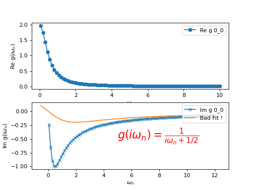
While one can use the regular matplotlib subfigure to make multi-panel figures, subplots makes it a bit more pythonic:
from triqs.gf import *
from triqs.gf.descriptors import Omega
g = GfImFreq(indices = [1], beta = 50, n_points = 1000, name = "g")
g << inverse( Omega + 0.5 )

# open 2 panels top (t) and bottom (b)
from triqs.plot.mpl_interface import subplots
f, (t,b) = subplots( 2,1)

#plot ...
t.oplot(g.real, '-o', x_window = (0,10) )
b.oplot(g.imag, '-x', x_window = (0,12) )
b.oplot( lambda om : -om*0.8/(om*om + 4), name = "Bad Fit !")
b.text(5,-0.5, r'$g(i\omega_n) = \frac{1}{i \omega_n + 1/2} $', size = 20, color='r')

Plot protocol [Advanced]
What do we need to implement to plot an object ? Simply a little _plot_ method that reduces the object to a set of curves. This section describes the conventions on this function.
As soon as an object defines this method, it can be plotted by the oplot function of triqs.plot.mpl_interface. See example below.
- triqs.plot._plot_(OptionsDict)
OptionDict is a dictionary of options.
Warning
The method _plot_ must consume the options it uses (using e.g. the pop method of dict).
Other options will be passed to matplotlib, so leaving spurious options here will lead to errors.
- rtype:
a list of dict representing one curve each. These dict must have the following fields:
xdata: A 1-dimensional numpy array describing the x-axis points
ydata: A 1-dimensional numpy array describing the y-axis points
label: Label of the curve for the legend of the graph
and optionally:
xlabel: a label for the x axis. The last object plotted will overrule the previous ones.
ylabel: a label for the y axis. The last object plotted will overrule the previous ones.
Example
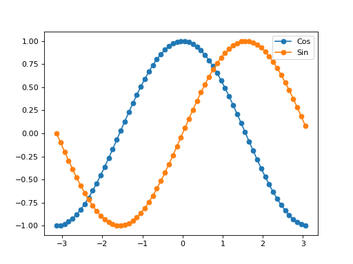
Here’s a simple example to illustrate the protocol:
import numpy

class myObject:
  def _plot_(self, options):
    PI = numpy.pi
    xdata = numpy.arange(-PI,PI,0.1)
    ydata1 = numpy.cos(xdata)
    ydata2 = numpy.sin(xdata)
    return( [
              {'xdata': xdata, 'ydata': ydata1, 'label': 'Cos'},
              {'xdata': xdata, 'ydata': ydata2, 'label': 'Sin'}
            ] )

X = myObject()

from triqs.plot.mpl_interface import oplot
oplot(X,'-o')

Example with options
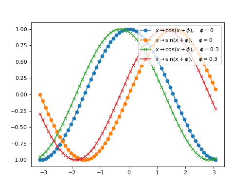
A little bit more complex, with options. Note the use of the pop method of dict, which returns and removes the entry from the dict (with a default value). All other options that may be passed to the plot function must be added to the returned dict, using the dict update method for example, otherwise they will not be used.
import numpy

class myObject:
  def _plot_(self, options):
    PI = numpy.pi
    xdata = numpy.arange(-PI,PI,0.1)
    phi = options.pop('phi',0)      # Crucial : removes the entry from the dict
    ydata1 = numpy.cos(xdata + phi)
    ydata2 = numpy.sin(xdata + phi)
    dict1 = {'xdata': xdata, 'ydata': ydata1, 'label': r'$x \rightarrow \cos (x + \phi), \quad \phi = %s$'%phi}
    dict2 = {'xdata': xdata, 'ydata': ydata2, 'label': r'$x \rightarrow \sin (x + \phi), \quad \phi = %s$'%phi}
    dict1.update(options)
    dict2.update(options)
    return [dict1, dict2]

X = myObject()

from triqs.plot.mpl_interface import oplot
oplot(X,'-o')
oplot(X,'-x', phi = 0.3)
