[GfReFreq] Retarded Green’s function in real frequencies

Reference

class triqs.gf.GfReFreq(**kw)[source]

Parameters (KEYWORD argument ONLY)

mesh: MeshReFreq, optional: The mesh of the Green function If not present, it will be constructed from the parameters beta, [n_points], [statistic]
data: numpy.array, optional: The data of the Gf. Must be of dimension mesh.rank + target_rank. Incompatible with target_shape
target_shape: list of int, optional: Shape of the target space. Incompatible with data
is_real: bool: Is the Green function real valued ? If true, and target_shape is set, the data will be real. No effect with the parameter data.
name: str: The name of the Green function. For plotting.

conjugate()

Conjugate of the Greens function.

Returns:: G – Conjugate of the Greens function.
Return type:: Gf (copy)

set_from_fourier(*args, **kw)

Fills self with the Fourier transform of g_in

Signature(gf_view<imtime,scalar_valued> g_out, gf_view<imfreq,scalar_valued> g_in) -> None: Fills self with the Fourier transform of g_in
Signature(block_gf_view<imtime,scalar_valued> g_out, block_gf_view<imfreq,scalar_valued> g_in) -> None: Fills self with the Fourier transform of g_in
Signature(block2_gf_view<imtime,scalar_valued> g_out, block2_gf_view<imfreq,scalar_valued> g_in) -> None: Fills self with the Fourier transform of g_in
Signature(gf_view<imtime,scalar_valued> g_out, gf_view<imfreq,scalar_valued> g_in, array_const_view<dcomplex,1+scalar_valued::rank> known_moments) -> None: Fills self with the Fourier transform of g_in with known high-frequency moments
Signature(gf_view<imfreq,scalar_valued> g_out, gf_view<imtime,scalar_valued> g_in) -> None: Fills self with the Fourier transform of g_in
Signature(gf_view<imfreq,scalar_valued> g_out, gf_view<imtime,typename scalar_valued::real_t> g_in) -> None: Fills self with the Fourier transform of g_in
Signature(block_gf_view<imfreq,scalar_valued> g_out, block_gf_view<imtime,scalar_valued> g_in) -> None: Fills self with the Fourier transform of g_in
Signature(block_gf_view<imfreq,scalar_valued> g_out, block_gf_view<imtime,typename scalar_valued::real_t> g_in) -> None: Fills self with the Fourier transform of g_in
Signature(block2_gf_view<imfreq,scalar_valued> g_out, block2_gf_view<imtime,scalar_valued> g_in) -> None: Fills self with the Fourier transform of g_in
Signature(block2_gf_view<imfreq,scalar_valued> g_out, block2_gf_view<imtime,typename scalar_valued::real_t> g_in) -> None: Fills self with the Fourier transform of g_in
Signature(gf_view<imfreq,scalar_valued> g_out, gf_view<imtime,scalar_valued> g_in, array_const_view<dcomplex,1+scalar_valued::rank> known_moments) -> None: Fills self with the Fourier transform of g_in with known high-frequency moments
Signature(gf_view<retime,scalar_valued> g_out, gf_view<refreq,scalar_valued> g_in) -> None: Fills self with the Fourier transform of g_in
Signature(block_gf_view<retime,scalar_valued> g_out, block_gf_view<refreq,scalar_valued> g_in) -> None: Fills self with the Fourier transform of g_in
Signature(block2_gf_view<retime,scalar_valued> g_out, block2_gf_view<refreq,scalar_valued> g_in) -> None: Fills self with the Fourier transform of g_in
Signature(gf_view<retime,scalar_valued> g_out, gf_view<refreq,scalar_valued> g_in, array_const_view<dcomplex,1+scalar_valued::rank> known_moments) -> None: Fills self with the Fourier transform of g_in with known high-frequency moments
Signature(gf_view<refreq,scalar_valued> g_out, gf_view<retime,scalar_valued> g_in) -> None: Fills self with the Fourier transform of g_in
Signature(gf_view<refreq,scalar_valued> g_out, gf_view<retime,typename scalar_valued::real_t> g_in) -> None: Fills self with the Fourier transform of g_in
Signature(block_gf_view<refreq,scalar_valued> g_out, block_gf_view<retime,scalar_valued> g_in) -> None: Fills self with the Fourier transform of g_in
Signature(block_gf_view<refreq,scalar_valued> g_out, block_gf_view<retime,typename scalar_valued::real_t> g_in) -> None: Fills self with the Fourier transform of g_in
Signature(block2_gf_view<refreq,scalar_valued> g_out, block2_gf_view<retime,scalar_valued> g_in) -> None: Fills self with the Fourier transform of g_in
Signature(block2_gf_view<refreq,scalar_valued> g_out, block2_gf_view<retime,typename scalar_valued::real_t> g_in) -> None: Fills self with the Fourier transform of g_in
Signature(gf_view<refreq,scalar_valued> g_out, gf_view<retime,scalar_valued> g_in, array_const_view<dcomplex,1+scalar_valued::rank> known_moments) -> None: Fills self with the Fourier transform of g_in with known high-frequency moments
Signature(gf_view<cyclat,scalar_valued> g_out, gf_view<brzone,scalar_valued> g_in) -> None: Fills self with the Fourier transform of g_in
Signature(block_gf_view<cyclat,scalar_valued> g_out, block_gf_view<brzone,scalar_valued> g_in) -> None: Fills self with the Fourier transform of g_in
Signature(block2_gf_view<cyclat,scalar_valued> g_out, block2_gf_view<brzone,scalar_valued> g_in) -> None: Fills self with the Fourier transform of g_in
Signature(gf_view<brzone,scalar_valued> g_out, gf_view<cyclat,scalar_valued> g_in) -> None: Fills self with the Fourier transform of g_in
Signature(block_gf_view<brzone,scalar_valued> g_out, block_gf_view<cyclat,scalar_valued> g_in) -> None: Fills self with the Fourier transform of g_in
Signature(block2_gf_view<brzone,scalar_valued> g_out, block2_gf_view<cyclat,scalar_valued> g_in) -> None: Fills self with the Fourier transform of g_in
Signature(gf_view<imtime,tensor_valued<1>> g_out, gf_view<imfreq,tensor_valued<1>> g_in) -> None: Fills self with the Fourier transform of g_in
Signature(block_gf_view<imtime,tensor_valued<1>> g_out, block_gf_view<imfreq,tensor_valued<1>> g_in) -> None: Fills self with the Fourier transform of g_in
Signature(block2_gf_view<imtime,tensor_valued<1>> g_out, block2_gf_view<imfreq,tensor_valued<1>> g_in) -> None: Fills self with the Fourier transform of g_in
Signature(gf_view<imtime,tensor_valued<1>> g_out, gf_view<imfreq,tensor_valued<1>> g_in, array_const_view<dcomplex,1+tensor_valued<1>::rank> known_moments) -> None: Fills self with the Fourier transform of g_in with known high-frequency moments
Signature(gf_view<imfreq,tensor_valued<1>> g_out, gf_view<imtime,tensor_valued<1>> g_in) -> None: Fills self with the Fourier transform of g_in
Signature(gf_view<imfreq,tensor_valued<1>> g_out, gf_view<imtime,typename tensor_valued<1>::real_t> g_in) -> None: Fills self with the Fourier transform of g_in
Signature(block_gf_view<imfreq,tensor_valued<1>> g_out, block_gf_view<imtime,tensor_valued<1>> g_in) -> None: Fills self with the Fourier transform of g_in
Signature(block_gf_view<imfreq,tensor_valued<1>> g_out, block_gf_view<imtime,typename tensor_valued<1>::real_t> g_in) -> None: Fills self with the Fourier transform of g_in
Signature(block2_gf_view<imfreq,tensor_valued<1>> g_out, block2_gf_view<imtime,tensor_valued<1>> g_in) -> None: Fills self with the Fourier transform of g_in
Signature(block2_gf_view<imfreq,tensor_valued<1>> g_out, block2_gf_view<imtime,typename tensor_valued<1>::real_t> g_in) -> None: Fills self with the Fourier transform of g_in
Signature(gf_view<imfreq,tensor_valued<1>> g_out, gf_view<imtime,tensor_valued<1>> g_in, array_const_view<dcomplex,1+tensor_valued<1>::rank> known_moments) -> None: Fills self with the Fourier transform of g_in with known high-frequency moments
Signature(gf_view<retime,tensor_valued<1>> g_out, gf_view<refreq,tensor_valued<1>> g_in) -> None: Fills self with the Fourier transform of g_in
Signature(block_gf_view<retime,tensor_valued<1>> g_out, block_gf_view<refreq,tensor_valued<1>> g_in) -> None: Fills self with the Fourier transform of g_in
Signature(block2_gf_view<retime,tensor_valued<1>> g_out, block2_gf_view<refreq,tensor_valued<1>> g_in) -> None: Fills self with the Fourier transform of g_in
Signature(gf_view<retime,tensor_valued<1>> g_out, gf_view<refreq,tensor_valued<1>> g_in, array_const_view<dcomplex,1+tensor_valued<1>::rank> known_moments) -> None: Fills self with the Fourier transform of g_in with known high-frequency moments
Signature(gf_view<refreq,tensor_valued<1>> g_out, gf_view<retime,tensor_valued<1>> g_in) -> None: Fills self with the Fourier transform of g_in
Signature(gf_view<refreq,tensor_valued<1>> g_out, gf_view<retime,typename tensor_valued<1>::real_t> g_in) -> None: Fills self with the Fourier transform of g_in
Signature(block_gf_view<refreq,tensor_valued<1>> g_out, block_gf_view<retime,tensor_valued<1>> g_in) -> None: Fills self with the Fourier transform of g_in
Signature(block_gf_view<refreq,tensor_valued<1>> g_out, block_gf_view<retime,typename tensor_valued<1>::real_t> g_in) -> None: Fills self with the Fourier transform of g_in
Signature(block2_gf_view<refreq,tensor_valued<1>> g_out, block2_gf_view<retime,tensor_valued<1>> g_in) -> None: Fills self with the Fourier transform of g_in
Signature(block2_gf_view<refreq,tensor_valued<1>> g_out, block2_gf_view<retime,typename tensor_valued<1>::real_t> g_in) -> None: Fills self with the Fourier transform of g_in
Signature(gf_view<refreq,tensor_valued<1>> g_out, gf_view<retime,tensor_valued<1>> g_in, array_const_view<dcomplex,1+tensor_valued<1>::rank> known_moments) -> None: Fills self with the Fourier transform of g_in with known high-frequency moments
Signature(gf_view<cyclat,tensor_valued<1>> g_out, gf_view<brzone,tensor_valued<1>> g_in) -> None: Fills self with the Fourier transform of g_in
Signature(block_gf_view<cyclat,tensor_valued<1>> g_out, block_gf_view<brzone,tensor_valued<1>> g_in) -> None: Fills self with the Fourier transform of g_in
Signature(block2_gf_view<cyclat,tensor_valued<1>> g_out, block2_gf_view<brzone,tensor_valued<1>> g_in) -> None: Fills self with the Fourier transform of g_in
Signature(gf_view<brzone,tensor_valued<1>> g_out, gf_view<cyclat,tensor_valued<1>> g_in) -> None: Fills self with the Fourier transform of g_in
Signature(block_gf_view<brzone,tensor_valued<1>> g_out, block_gf_view<cyclat,tensor_valued<1>> g_in) -> None: Fills self with the Fourier transform of g_in
Signature(block2_gf_view<brzone,tensor_valued<1>> g_out, block2_gf_view<cyclat,tensor_valued<1>> g_in) -> None: Fills self with the Fourier transform of g_in
Signature(gf_view<imtime,matrix_valued> g_out, gf_view<imfreq,matrix_valued> g_in) -> None: Fills self with the Fourier transform of g_in
Signature(block_gf_view<imtime,matrix_valued> g_out, block_gf_view<imfreq,matrix_valued> g_in) -> None: Fills self with the Fourier transform of g_in
Signature(block2_gf_view<imtime,matrix_valued> g_out, block2_gf_view<imfreq,matrix_valued> g_in) -> None: Fills self with the Fourier transform of g_in
Signature(gf_view<imtime,matrix_valued> g_out, gf_view<imfreq,matrix_valued> g_in, array_const_view<dcomplex,1+matrix_valued::rank> known_moments) -> None: Fills self with the Fourier transform of g_in with known high-frequency moments
Signature(gf_view<imfreq,matrix_valued> g_out, gf_view<imtime,matrix_valued> g_in) -> None: Fills self with the Fourier transform of g_in
Signature(gf_view<imfreq,matrix_valued> g_out, gf_view<imtime,typename matrix_valued::real_t> g_in) -> None: Fills self with the Fourier transform of g_in
Signature(block_gf_view<imfreq,matrix_valued> g_out, block_gf_view<imtime,matrix_valued> g_in) -> None: Fills self with the Fourier transform of g_in
Signature(block_gf_view<imfreq,matrix_valued> g_out, block_gf_view<imtime,typename matrix_valued::real_t> g_in) -> None: Fills self with the Fourier transform of g_in
Signature(block2_gf_view<imfreq,matrix_valued> g_out, block2_gf_view<imtime,matrix_valued> g_in) -> None: Fills self with the Fourier transform of g_in
Signature(block2_gf_view<imfreq,matrix_valued> g_out, block2_gf_view<imtime,typename matrix_valued::real_t> g_in) -> None: Fills self with the Fourier transform of g_in
Signature(gf_view<imfreq,matrix_valued> g_out, gf_view<imtime,matrix_valued> g_in, array_const_view<dcomplex,1+matrix_valued::rank> known_moments) -> None: Fills self with the Fourier transform of g_in with known high-frequency moments
Signature(gf_view<retime,matrix_valued> g_out, gf_view<refreq,matrix_valued> g_in) -> None: Fills self with the Fourier transform of g_in
Signature(block_gf_view<retime,matrix_valued> g_out, block_gf_view<refreq,matrix_valued> g_in) -> None: Fills self with the Fourier transform of g_in
Signature(block2_gf_view<retime,matrix_valued> g_out, block2_gf_view<refreq,matrix_valued> g_in) -> None: Fills self with the Fourier transform of g_in
Signature(gf_view<retime,matrix_valued> g_out, gf_view<refreq,matrix_valued> g_in, array_const_view<dcomplex,1+matrix_valued::rank> known_moments) -> None: Fills self with the Fourier transform of g_in with known high-frequency moments
Signature(gf_view<refreq,matrix_valued> g_out, gf_view<retime,matrix_valued> g_in) -> None: Fills self with the Fourier transform of g_in
Signature(gf_view<refreq,matrix_valued> g_out, gf_view<retime,typename matrix_valued::real_t> g_in) -> None: Fills self with the Fourier transform of g_in
Signature(block_gf_view<refreq,matrix_valued> g_out, block_gf_view<retime,matrix_valued> g_in) -> None: Fills self with the Fourier transform of g_in
Signature(block_gf_view<refreq,matrix_valued> g_out, block_gf_view<retime,typename matrix_valued::real_t> g_in) -> None: Fills self with the Fourier transform of g_in
Signature(block2_gf_view<refreq,matrix_valued> g_out, block2_gf_view<retime,matrix_valued> g_in) -> None: Fills self with the Fourier transform of g_in
Signature(block2_gf_view<refreq,matrix_valued> g_out, block2_gf_view<retime,typename matrix_valued::real_t> g_in) -> None: Fills self with the Fourier transform of g_in
Signature(gf_view<refreq,matrix_valued> g_out, gf_view<retime,matrix_valued> g_in, array_const_view<dcomplex,1+matrix_valued::rank> known_moments) -> None: Fills self with the Fourier transform of g_in with known high-frequency moments
Signature(gf_view<cyclat,matrix_valued> g_out, gf_view<brzone,matrix_valued> g_in) -> None: Fills self with the Fourier transform of g_in
Signature(block_gf_view<cyclat,matrix_valued> g_out, block_gf_view<brzone,matrix_valued> g_in) -> None: Fills self with the Fourier transform of g_in
Signature(block2_gf_view<cyclat,matrix_valued> g_out, block2_gf_view<brzone,matrix_valued> g_in) -> None: Fills self with the Fourier transform of g_in
Signature(gf_view<brzone,matrix_valued> g_out, gf_view<cyclat,matrix_valued> g_in) -> None: Fills self with the Fourier transform of g_in
Signature(block_gf_view<brzone,matrix_valued> g_out, block_gf_view<cyclat,matrix_valued> g_in) -> None: Fills self with the Fourier transform of g_in
Signature(block2_gf_view<brzone,matrix_valued> g_out, block2_gf_view<cyclat,matrix_valued> g_in) -> None: Fills self with the Fourier transform of g_in
Signature(gf_view<imtime,tensor_valued<3>> g_out, gf_view<imfreq,tensor_valued<3>> g_in) -> None: Fills self with the Fourier transform of g_in
Signature(block_gf_view<imtime,tensor_valued<3>> g_out, block_gf_view<imfreq,tensor_valued<3>> g_in) -> None: Fills self with the Fourier transform of g_in
Signature(block2_gf_view<imtime,tensor_valued<3>> g_out, block2_gf_view<imfreq,tensor_valued<3>> g_in) -> None: Fills self with the Fourier transform of g_in
Signature(gf_view<imtime,tensor_valued<3>> g_out, gf_view<imfreq,tensor_valued<3>> g_in, array_const_view<dcomplex,1+tensor_valued<3>::rank> known_moments) -> None: Fills self with the Fourier transform of g_in with known high-frequency moments
Signature(gf_view<imfreq,tensor_valued<3>> g_out, gf_view<imtime,tensor_valued<3>> g_in) -> None: Fills self with the Fourier transform of g_in
Signature(gf_view<imfreq,tensor_valued<3>> g_out, gf_view<imtime,typename tensor_valued<3>::real_t> g_in) -> None: Fills self with the Fourier transform of g_in
Signature(block_gf_view<imfreq,tensor_valued<3>> g_out, block_gf_view<imtime,tensor_valued<3>> g_in) -> None: Fills self with the Fourier transform of g_in
Signature(block_gf_view<imfreq,tensor_valued<3>> g_out, block_gf_view<imtime,typename tensor_valued<3>::real_t> g_in) -> None: Fills self with the Fourier transform of g_in
Signature(block2_gf_view<imfreq,tensor_valued<3>> g_out, block2_gf_view<imtime,tensor_valued<3>> g_in) -> None: Fills self with the Fourier transform of g_in
Signature(block2_gf_view<imfreq,tensor_valued<3>> g_out, block2_gf_view<imtime,typename tensor_valued<3>::real_t> g_in) -> None: Fills self with the Fourier transform of g_in
Signature(gf_view<imfreq,tensor_valued<3>> g_out, gf_view<imtime,tensor_valued<3>> g_in, array_const_view<dcomplex,1+tensor_valued<3>::rank> known_moments) -> None: Fills self with the Fourier transform of g_in with known high-frequency moments
Signature(gf_view<retime,tensor_valued<3>> g_out, gf_view<refreq,tensor_valued<3>> g_in) -> None: Fills self with the Fourier transform of g_in
Signature(block_gf_view<retime,tensor_valued<3>> g_out, block_gf_view<refreq,tensor_valued<3>> g_in) -> None: Fills self with the Fourier transform of g_in
Signature(block2_gf_view<retime,tensor_valued<3>> g_out, block2_gf_view<refreq,tensor_valued<3>> g_in) -> None: Fills self with the Fourier transform of g_in
Signature(gf_view<retime,tensor_valued<3>> g_out, gf_view<refreq,tensor_valued<3>> g_in, array_const_view<dcomplex,1+tensor_valued<3>::rank> known_moments) -> None: Fills self with the Fourier transform of g_in with known high-frequency moments
Signature(gf_view<refreq,tensor_valued<3>> g_out, gf_view<retime,tensor_valued<3>> g_in) -> None: Fills self with the Fourier transform of g_in
Signature(gf_view<refreq,tensor_valued<3>> g_out, gf_view<retime,typename tensor_valued<3>::real_t> g_in) -> None: Fills self with the Fourier transform of g_in
Signature(block_gf_view<refreq,tensor_valued<3>> g_out, block_gf_view<retime,tensor_valued<3>> g_in) -> None: Fills self with the Fourier transform of g_in
Signature(block_gf_view<refreq,tensor_valued<3>> g_out, block_gf_view<retime,typename tensor_valued<3>::real_t> g_in) -> None: Fills self with the Fourier transform of g_in
Signature(block2_gf_view<refreq,tensor_valued<3>> g_out, block2_gf_view<retime,tensor_valued<3>> g_in) -> None: Fills self with the Fourier transform of g_in
Signature(block2_gf_view<refreq,tensor_valued<3>> g_out, block2_gf_view<retime,typename tensor_valued<3>::real_t> g_in) -> None: Fills self with the Fourier transform of g_in
Signature(gf_view<refreq,tensor_valued<3>> g_out, gf_view<retime,tensor_valued<3>> g_in, array_const_view<dcomplex,1+tensor_valued<3>::rank> known_moments) -> None: Fills self with the Fourier transform of g_in with known high-frequency moments
Signature(gf_view<cyclat,tensor_valued<3>> g_out, gf_view<brzone,tensor_valued<3>> g_in) -> None: Fills self with the Fourier transform of g_in
Signature(block_gf_view<cyclat,tensor_valued<3>> g_out, block_gf_view<brzone,tensor_valued<3>> g_in) -> None: Fills self with the Fourier transform of g_in
Signature(block2_gf_view<cyclat,tensor_valued<3>> g_out, block2_gf_view<brzone,tensor_valued<3>> g_in) -> None: Fills self with the Fourier transform of g_in
Signature(gf_view<brzone,tensor_valued<3>> g_out, gf_view<cyclat,tensor_valued<3>> g_in) -> None: Fills self with the Fourier transform of g_in
Signature(block_gf_view<brzone,tensor_valued<3>> g_out, block_gf_view<cyclat,tensor_valued<3>> g_in) -> None: Fills self with the Fourier transform of g_in
Signature(block2_gf_view<brzone,tensor_valued<3>> g_out, block2_gf_view<cyclat,tensor_valued<3>> g_in) -> None: Fills self with the Fourier transform of g_in
Signature(gf_view<imtime,tensor_valued<4>> g_out, gf_view<imfreq,tensor_valued<4>> g_in) -> None: Fills self with the Fourier transform of g_in
Signature(block_gf_view<imtime,tensor_valued<4>> g_out, block_gf_view<imfreq,tensor_valued<4>> g_in) -> None: Fills self with the Fourier transform of g_in
Signature(block2_gf_view<imtime,tensor_valued<4>> g_out, block2_gf_view<imfreq,tensor_valued<4>> g_in) -> None: Fills self with the Fourier transform of g_in
Signature(gf_view<imtime,tensor_valued<4>> g_out, gf_view<imfreq,tensor_valued<4>> g_in, array_const_view<dcomplex,1+tensor_valued<4>::rank> known_moments) -> None: Fills self with the Fourier transform of g_in with known high-frequency moments
Signature(gf_view<imfreq,tensor_valued<4>> g_out, gf_view<imtime,tensor_valued<4>> g_in) -> None: Fills self with the Fourier transform of g_in
Signature(gf_view<imfreq,tensor_valued<4>> g_out, gf_view<imtime,typename tensor_valued<4>::real_t> g_in) -> None: Fills self with the Fourier transform of g_in
Signature(block_gf_view<imfreq,tensor_valued<4>> g_out, block_gf_view<imtime,tensor_valued<4>> g_in) -> None: Fills self with the Fourier transform of g_in
Signature(block_gf_view<imfreq,tensor_valued<4>> g_out, block_gf_view<imtime,typename tensor_valued<4>::real_t> g_in) -> None: Fills self with the Fourier transform of g_in
Signature(block2_gf_view<imfreq,tensor_valued<4>> g_out, block2_gf_view<imtime,tensor_valued<4>> g_in) -> None: Fills self with the Fourier transform of g_in
Signature(block2_gf_view<imfreq,tensor_valued<4>> g_out, block2_gf_view<imtime,typename tensor_valued<4>::real_t> g_in) -> None: Fills self with the Fourier transform of g_in
Signature(gf_view<imfreq,tensor_valued<4>> g_out, gf_view<imtime,tensor_valued<4>> g_in, array_const_view<dcomplex,1+tensor_valued<4>::rank> known_moments) -> None: Fills self with the Fourier transform of g_in with known high-frequency moments
Signature(gf_view<retime,tensor_valued<4>> g_out, gf_view<refreq,tensor_valued<4>> g_in) -> None: Fills self with the Fourier transform of g_in
Signature(block_gf_view<retime,tensor_valued<4>> g_out, block_gf_view<refreq,tensor_valued<4>> g_in) -> None: Fills self with the Fourier transform of g_in
Signature(block2_gf_view<retime,tensor_valued<4>> g_out, block2_gf_view<refreq,tensor_valued<4>> g_in) -> None: Fills self with the Fourier transform of g_in
Signature(gf_view<retime,tensor_valued<4>> g_out, gf_view<refreq,tensor_valued<4>> g_in, array_const_view<dcomplex,1+tensor_valued<4>::rank> known_moments) -> None: Fills self with the Fourier transform of g_in with known high-frequency moments
Signature(gf_view<refreq,tensor_valued<4>> g_out, gf_view<retime,tensor_valued<4>> g_in) -> None: Fills self with the Fourier transform of g_in
Signature(gf_view<refreq,tensor_valued<4>> g_out, gf_view<retime,typename tensor_valued<4>::real_t> g_in) -> None: Fills self with the Fourier transform of g_in
Signature(block_gf_view<refreq,tensor_valued<4>> g_out, block_gf_view<retime,tensor_valued<4>> g_in) -> None: Fills self with the Fourier transform of g_in
Signature(block_gf_view<refreq,tensor_valued<4>> g_out, block_gf_view<retime,typename tensor_valued<4>::real_t> g_in) -> None: Fills self with the Fourier transform of g_in
Signature(block2_gf_view<refreq,tensor_valued<4>> g_out, block2_gf_view<retime,tensor_valued<4>> g_in) -> None: Fills self with the Fourier transform of g_in
Signature(block2_gf_view<refreq,tensor_valued<4>> g_out, block2_gf_view<retime,typename tensor_valued<4>::real_t> g_in) -> None: Fills self with the Fourier transform of g_in
Signature(gf_view<refreq,tensor_valued<4>> g_out, gf_view<retime,tensor_valued<4>> g_in, array_const_view<dcomplex,1+tensor_valued<4>::rank> known_moments) -> None: Fills self with the Fourier transform of g_in with known high-frequency moments
Signature(gf_view<cyclat,tensor_valued<4>> g_out, gf_view<brzone,tensor_valued<4>> g_in) -> None: Fills self with the Fourier transform of g_in
Signature(block_gf_view<cyclat,tensor_valued<4>> g_out, block_gf_view<brzone,tensor_valued<4>> g_in) -> None: Fills self with the Fourier transform of g_in
Signature(block2_gf_view<cyclat,tensor_valued<4>> g_out, block2_gf_view<brzone,tensor_valued<4>> g_in) -> None: Fills self with the Fourier transform of g_in
Signature(gf_view<brzone,tensor_valued<4>> g_out, gf_view<cyclat,tensor_valued<4>> g_in) -> None: Fills self with the Fourier transform of g_in
Signature(block_gf_view<brzone,tensor_valued<4>> g_out, block_gf_view<cyclat,tensor_valued<4>> g_in) -> None: Fills self with the Fourier transform of g_in
Signature(block2_gf_view<brzone,tensor_valued<4>> g_out, block2_gf_view<cyclat,tensor_valued<4>> g_in) -> None: Fills self with the Fourier transform of g_in

set_from_pade(*args, **kw)

Signature : (gf_view<refreq,scalar_valued> gw, gf_view<imfreq,scalar_valued> giw, int n_points = 100, float freq_offset = 0.0) -> None

Signature : (gf_view<refreq,tensor_valued<1>> gw, gf_view<imfreq,tensor_valued<1>> giw, int n_points = 100, float freq_offset = 0.0) -> None

Signature : (gf_view<refreq,matrix_valued> gw, gf_view<imfreq,matrix_valued> giw, int n_points = 100, float freq_offset = 0.0) -> None

Signature : (gf_view<refreq,tensor_valued<3>> gw, gf_view<imfreq,tensor_valued<3>> giw, int n_points = 100, float freq_offset = 0.0) -> None

Signature : (gf_view<refreq,tensor_valued<4>> gw, gf_view<imfreq,tensor_valued<4>> giw, int n_points = 100, float freq_offset = 0.0) -> None

transpose()

Take the transpose of a matrix valued Greens function.

Returns:: G – The transpose of the Greens function.
Return type:: Gf (copy)

Notes

Only implemented for single mesh matrix valued Greens functions.

Warning

Arguments of __init__() must be documented.

HDF5 data scheme

The GfReFreq (Format = “GfReFreq”) is decomposed in the following objects:

Name	Type	Meaning
Mesh	MeshGf	The mesh
Data	3d numpy of complex	Data[n,i1,i2] is the element of the Green function where: n is the frequency index i1, i2 are the indices
IndicesL,IndicesR	string	The Python repr of the indices, e.g. (1,2), or (1,) repr(this_string) reproduces the indices
Name	string	Name of the Green function block
Note	string	Note

Examples

import numpy as np
from triqs.gf import GfReFreq, SemiCircular

g = GfReFreq(indices = ['eg1', 'eg2'], window = (-5, 5), n_points = 1000, name = "egBlock")

g['eg1','eg1'] = SemiCircular(half_bandwidth = 1)
g['eg2','eg2'] = SemiCircular(half_bandwidth = 2)

from triqs.plot.mpl_interface import oplot
oplot(g['eg1','eg1'], '-o', mode = 'S')  # S : spectral function 
oplot(g['eg2','eg2'], '-x', mode = 'S')

Note that g is a retarded Green’s function.

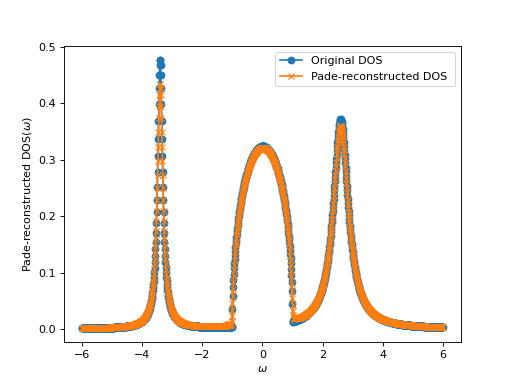
The next example demonstrates how a real frequency Green’s function can be reconstructed from an imaginary frequency counterpart using set_from_pade() method.

import numpy
from math import pi
from cmath import sqrt, log
from triqs.gf import *
from triqs.gf.descriptors import Function

beta = 100  # Inverse temperature
L = 101     # Number of Matsubara frequencies used in the Pade approximation
eta = 0.01  # Imaginary frequency shift

## Test Green's functions ##

# Two Lorentzians
def GLorentz(z):
    return 0.7/(z-2.6+0.3*1j) + 0.3/(z+3.4+0.1*1j)

# Semicircle
def GSC(z):
    return 2.0*(z + sqrt(1-z**2)*(log(1-z) - log(-1+z))/pi)

# A superposition of GLorentz(z) and GSC(z) with equal weights
def G(z):
    return 0.5*GLorentz(z) + 0.5*GSC(z)

# Matsubara GF
gm = GfImFreq(indices = [0], beta = beta, name = "gm", n_points=2000)
gm << Function(G)

# Real frequency BlockGf(documentation/manual/triqs)
gr = GfReFreq(indices = [0], window = (-5.995, 5.995), n_points = 1200, name = "gr")
gr << Function(G)

# Analytic continuation of gm
g_pade = GfReFreq(indices = [0], window = (-5.995, 5.995), n_points = 1200, name = "g_pade")
g_pade.set_from_pade(gm, n_points = L, freq_offset = eta)

# Comparison plot
from triqs.plot.mpl_interface import oplot
oplot(gr[0,0], '-o', mode = 'S', name = "Original DOS")
oplot(g_pade[0,0], '-x', mode = 'S', name = "Pade-reconstructed DOS")

../../../../../../_images/green_pade.png